Making Electronic Oscillation Performable
Section I · Theory
Build the modelSound, history, and the mathematics that connects them.Chapter contract
Prerequisites. Chapter 1 invariants, algebraic rearrangement, and the ability to distinguish pitch from amplitude while listening.
By the end of this chapter, you should be able to:
- predict how inductance and capacitance affect an LC resonant frequency;
- trace energy exchange and amplitude trajectories in passive and maintained LC tanks;
- predict and hear constructive and destructive summation;
- separate the variable RF oscillator from the audible difference frequency;
- derive sum and difference components from nonlinear multiplication;
- distinguish linear beating from heterodyne frequency conversion;
- describe independent pitch and amplitude gesture mappings;
- distinguish vibrato, portamento, glissando, and articulation;
- compare the theremin and Ondes Martenot as different solutions to performability;
- solve LC-ratio, frequency-difference, cents, interpolation, and phase-accumulation problems;
- explain every numbered formula from its adjacent plot;
- extend the Chapter 1 browser oscillator into a gesture and articulation renderer.
The problem: how does a body control an invisible oscillator?
Hold one hand near a pitch antenna and the other near a volume loop. Move either hand without touching the instrument. Pitch or loudness changes continuously.
How can body position control an oscillator without keys or contact?
Lev Termen developed his instrument around 1919–20. Public demonstrations followed by 1920–21, depending on which event a source dates. His instrument turned the performer’s proximity into control of electronic oscillators. It became known as the theremin. Because “first electronic instrument” depends on whether electromechanical predecessors, prototypes, and commercial availability are included, this book uses the narrower description one of the earliest fully electronic musical instruments (Verhulst n.d.b; Skeldon et al. 1998; Alonso-Pérez and Batista n.d.).
Long description. A performer stands between a straight vertical antenna on the right and a horizontal loop on the left. The right hand moves toward and away from the straight antenna to alter pitch. The left hand moves above the loop to alter amplitude. The diagram abstracts the control relationships without reproducing a rights-sensitive historical photograph.
The theremin joins three models:
- a resonant electronic oscillator;
- a nonlinear frequency converter;
- a learned gesture-to-music mapping.
Sustained LC oscillation
LC means inductor–capacitor. The letter stands for inductance, and stands for capacitance. An ideal LC resonator exchanges energy between the capacitor’s electric field and the inductor’s magnetic field. Its natural frequency is:
| Symbol | Meaning | Unit |
|---|---|---|
| inductance | henries | |
| effective capacitance | farads | |
| resonant frequency | hertz |

Long description. The curve falls from about 712 kHz at 50 pF toward 225 kHz at 500 pF. Markers show 503.3 kHz at 100 pF and 251.6 kHz at 400 pF. Quadrupling capacitance halves frequency when inductance stays fixed.
A real oscillator adds active feedback to replace losses. Without it, an idealized LC tank is only a resonator and a real one rings down.
How an LC tank exchanges energy
A tank circuit connects an inductor and capacitor so energy can move between two storage forms. Start by charging the capacitor, then let it discharge through the inductor:
- The charged capacitor stores energy in its electric field. Current is initially zero.
- The capacitor discharges. Current through the inductor rises, so magnetic-field energy grows.
- When the capacitor reaches zero charge, inductor current is largest. The collapsing magnetic field keeps current moving.
- That current charges the capacitor with opposite polarity. The exchange then reverses and repeats.
Capacitor charge and inductor current reach their extrema one quarter cycle apart. Their values change sign, but ideal total stored energy stays constant. Real wire resistance, capacitor loss, and radiation remove some energy on every cycle. Damping is this loss of oscillation amplitude over time (Electronics Tutorials n.d.).
An amplitude trajectory is the path a signal’s level takes through time. The tank makes three trajectories easy to compare:
| Model | Amplitude trajectory | What it sounds like at an audible frequency |
|---|---|---|
| Ideal lossless tank | Constant forever | A steady sine wave |
| Passive real tank | Falls toward zero | A ringing tone that fades away |
| Active oscillator | Rises from startup, then settles when controlled feedback balances loss | A tone that stabilizes; excess gain eventually clips and adds distortion |
The complete oscillator therefore needs a frequency-selective tank, an amplifier, and positive feedback returned with the required phase. Startup requires loop gain above one. A stable sustained state replaces about as much energy as the tank loses. Too little feedback decays. Too much grows until circuit limits reshape the waveform (Electronics Tutorials n.d.).
TANK CIRCUIT PLAYGROUND
Exchange energy, lose it, then replace it
Choose audible-scale component values. Compare a passive tank ringing down with a teaching oscillator that starts, replaces the loss, and settles.
With L at 100 mH and C at 10.0 microfarads, resonance is 159.2 Hz. Capacitor charge and inductor current exchange energy one quarter-cycle apart. The passive amplitude trajectory decays with a 1.2-second time constant. The simplified active trajectory rises with an 80-millisecond startup time constant, then settles.
Hearing safety. Start with a low playback level. These component values deliberately place resonance in the audible range. Theremin pitch tanks use much smaller capacitances and operate at radio frequencies.
Try these checks
- Double capacitance. Predict whether frequency rises or falls before reading the result.
- Shorten the decay time. Listen and watch the amplitude trajectory lose energy faster.
- Compare passive and maintained playback. Frequency stays fixed while one amplitude decays and the other rises, then settles.
- Explain why the tank alone rings down but the complete oscillator can continue.
Read the exact source running this playground
This TypeScript implements Equation 2.1, passive loss, a simplified active startup-to-steady envelope, energy-exchange traces, and both listening examples.
export const SAMPLE_RATE = 48_000;
const TAU = 2 * Math.PI;

export function lcFrequency(inductanceMillihenries: number, capacitanceMicrofarads: number) {
  const inductanceHenries = inductanceMillihenries / 1000;
  const capacitanceFarads = capacitanceMicrofarads / 1_000_000;
  return 1 / (TAU * Math.sqrt(inductanceHenries * capacitanceFarads));
}

export function ringEnvelope(timeSeconds: number, decaySeconds: number, maintained = false) {
  const time = Math.max(0, timeSeconds);
  if (maintained) return 1 - Math.exp(-time / 0.08);
  return Math.exp(-time / Math.max(0.01, decaySeconds));
}

export function tankTrace(
  inductanceMillihenries: number,
  capacitanceMicrofarads: number,
  decaySeconds: number,
  seconds: number,
  points = 480
) {
  const frequencyHz = lcFrequency(inductanceMillihenries, capacitanceMicrofarads);
  return Array.from({ length: points }, (_, index) => {
    const timeSeconds = seconds * index / (points - 1);
    const envelope = ringEnvelope(timeSeconds, decaySeconds);
    const phase = TAU * frequencyHz * timeSeconds;
    return {
      timeSeconds,
      capacitorCharge: envelope * Math.cos(phase),
      inductorCurrent: envelope * Math.sin(phase),
      envelope
    };
  });
}

export function renderTank(
  inductanceMillihenries: number,
  capacitanceMicrofarads: number,
  decaySeconds: number,
  maintained: boolean,
  seconds = 2.5
) {
  const frequencyHz = lcFrequency(inductanceMillihenries, capacitanceMicrofarads);
  const frameCount = Math.round(seconds * SAMPLE_RATE);
  const fadeFrames = Math.round(0.012 * SAMPLE_RATE);
  const output = new Float32Array(frameCount);

  for (let frame = 0; frame < frameCount; frame++) {
    const timeSeconds = frame / SAMPLE_RATE;
    const edgeFade = Math.min(1, frame / fadeFrames, (frameCount - 1 - frame) / fadeFrames);
    output[frame] = 0.18 * edgeFade * ringEnvelope(timeSeconds, decaySeconds, maintained)
      * Math.sin(TAU * frequencyHz * timeSeconds);
  }

  return output;
}
Hold fixed and increase . Frequency falls:
The performer’s hand and body contribute a small distributed capacitance involving the antenna, instrument ground, room, and nearby objects. Distributed means that the electric field and its charge-storage effect spread across several physical paths instead of living in one component. A picofarad, abbreviated pF, is one trillionth of a farad. Reported hand-motion changes are commonly fractions of a picofarad to a few picofarads (Skeldon et al. 1998; Alonso-Pérez and Batista n.d.).
Long description. A performer stands left of a vertical pitch antenna. Dashed paths connect the hand to the antenna, the body to the instrument reference, the antenna to the chassis, and the antenna to a nearby object. The changing performer paths join fixed room and instrument paths to form one effective capacitance.
Diagram provenance. Project-authored conceptual SVG based on the distributed-capacitance discussions by Skeldon and by Alonso-Pérez and Batista. It is a signal explanation, not a literal map of field strength or a circuit-construction diagram.
Instrument ground here means the circuit’s electrical reference and return path. It does not require a separate earth stake. The room, floor, chassis, performer, and nearby objects establish a baseline capacitance. Hand motion changes part of that total. Calibration absorbs much of the baseline so the small changing part can control pitch.
A parallel-plate model gives one useful direction: bringing conductive surfaces closer usually increases capacitance. A hand and rod are not parallel plates, however. Their curved shapes produce fringe fields, and the performer’s body participates in the return path. Use the plate idea to predict direction, not to calculate an exact theremin value.
Long description. The left panel places a hand farther from the antenna and labels the teaching model 100 pF and 503.3 kHz. The right panel moves the hand nearer and labels 101 pF and 500.8 kHz. A bottom arrow states that smaller distance raises effective capacitance and lowers the variable radio-frequency oscillator.
Diagram provenance. Project-authored calculation from Equation 2.1 with inductance fixed at 1 mH. The one-picofarad change is an illustrative teaching case within the cited scale of reported changes. It is not a measurement of a named theremin.
RF frequency is not audible pitch
Approaching the pitch antenna increases effective capacitance and lowers the variable radio-frequency oscillator’s own frequency. Yet the heard pitch can rise. Why? The output is not that RF oscillator directly. The instrument produces the difference between a variable RF oscillator and a fixed RF oscillator. Depending on how the pair is tuned, lowering the variable oscillator can increase their separation.
Confusing RF frequency with audible difference frequency is a common conceptual failure.
Heterodyning: make a small difference audible
Start with 500 and 501 kHz:
difference: 1 kHz
sum:        1001 kHz
A nonlinear mixer creates both components. A low-pass filter keeps the audible 1 kHz difference and rejects the RF sum.
Let the two oscillators be
The mixer multiplies them. The product-to-sum identity gives

Long description. The top panel overlays the two inputs. The middle panel shows their product and its slow 1.5 difference component. The bottom spectrum has lines at 1.5 and 21.5; the shaded low-pass region keeps only the difference.
Figure provenance. Author-generated by
assets/figures/src/ch02_heterodyne.py. Frequencies are
scaled so individual oscillations remain visible.
Therefore,

Long description. The upper V-shaped curve shows absolute difference falling to zero when both oscillators equal 500 kHz, then rising again. The lower line shows the sum increasing from 998 to 1002 kHz.
Circuit frequencies differ among designs. The 500/501 kHz pair is a teaching example, not a universal theremin specification (Skeldon et al. 1998; Alonso-Pérez and Batista n.d.).
Constructive and destructive summation
Play two equal 220 Hz sine waves. Frequency and amplitude match. Only relative phase changes:
0° apart:   crest + crest       → double amplitude
90° apart:  partial alignment   → √2 times one-wave amplitude
180° apart: crest + trough      → ideal cancellation
Constructive summation, also called constructive interference, occurs when aligned wave values reinforce one another. The ideal 0° pair keeps the same 220 Hz pitch and sine-wave timbre, but its peak amplitude doubles. Relative to either input alone, that is about 6.02 dB greater peak level. Destructive summation occurs when opposite values subtract. At 180°, two perfectly matched waves cancel to digital silence (Smith 2011; Puckette 2007).
| Relative phase | Peak ratio versus one wave | Ideal sound |
|---|---|---|
| 0° | 2.000 | Same pitch, clearly louder |
| 90° | 1.414 | Same pitch, partly reinforced |
| 180° | 0.000 | Silence |
Point to note. Constructive and destructive summation change the level of this matched-frequency result. They do not create a new sum-frequency or difference-frequency spectrum line. Those new components require nonlinear mixing.
Exact cancellation is a strict model boundary. Frequency, amplitude, waveform, timing, and listening position must match. A small mismatch leaves a quiet residue. Keep playback level low before comparing the louder constructive case. The phase-summation playground lets you hear one wave, reinforcement, partial cancellation, and ideal cancellation without normalizing their levels.
PHASE-SUMMATION PLAYGROUND
Hear phase become level
Keep two 220 Hz sine waves equal. Move only their relative phase, then hear their unnormalized sum.
Peak ratio: 2.000+6.02 dB versus one wave
Two equal 220 Hz sine waves are aligned. Their sum keeps the 220 Hz pitch and has twice the peak amplitude, 6.02 dB above one wave.
Hearing safety. Start quietly. The 0° sum is intentionally 6.02 dB above one input because the examples are not loudness-normalized.
Try these checks
- At 0°, identify the unchanged pitch and increased level.
- At 90°, predict the 1.414 peak ratio and +3.01 dB result.
- At 180°, explain why ideal playback is silence rather than a new tone.
- Move one degree away from 180°. Listen for the small residual that returns.
Read the exact source running this playground
This TypeScript calculates the phase-dependent peak ratio and renders the one-wave and two-wave listening examples.
export const SAMPLE_RATE = 48_000;
const TAU = 2 * Math.PI;

export function phaseSumGain(phaseDegrees: number) {
  const gain = 2 * Math.abs(Math.cos(phaseDegrees * Math.PI / 360));
  return gain < 1e-12 ? 0 : gain;
}

export function phaseSumWaveforms(phaseDegrees: number, points = 480) {
  const phaseRadians = phaseDegrees * Math.PI / 180;
  return Array.from({ length: points }, (_, index) => {
    const phase = TAU * 3 * index / (points - 1);
    const first = Math.sin(phase);
    const second = Math.sin(phase + phaseRadians);
    return { first, second, sum: first + second };
  });
}

export function renderSingleTone(frequencyHz = 220, seconds = 1.4) {
  const frameCount = Math.round(seconds * SAMPLE_RATE);
  const fadeFrames = Math.round(0.012 * SAMPLE_RATE);
  const output = new Float32Array(frameCount);

  for (let frame = 0; frame < frameCount; frame++) {
    const edgeFade = Math.min(1, frame / fadeFrames, (frameCount - 1 - frame) / fadeFrames);
    output[frame] = 0.09 * edgeFade * Math.sin(TAU * frequencyHz * frame / SAMPLE_RATE);
  }
  return output;
}

export function renderPhaseSum(phaseDegrees: number, frequencyHz = 220, seconds = 1.4) {
  const frameCount = Math.round(seconds * SAMPLE_RATE);
  const fadeFrames = Math.round(0.012 * SAMPLE_RATE);
  const phaseRadians = phaseDegrees * Math.PI / 180;
  const output = new Float32Array(frameCount);

  for (let frame = 0; frame < frameCount; frame++) {
    const phase = TAU * frequencyHz * frame / SAMPLE_RATE;
    const edgeFade = Math.min(1, frame / fadeFrames, (frameCount - 1 - frame) / fadeFrames);
    output[frame] = 0.09 * edgeFade * (Math.sin(phase) + Math.sin(phase + phaseRadians));
  }
  return output;
}
Beats are related but not identical
When frequencies differ slightly, their relative phase keeps moving. The waves pass repeatedly through constructive and destructive regions, so loudness rises and falls. Add the same two sinusoids instead of multiplying them:

Long description. The upper panel shows a fast linear sum bounded by a slow dashed envelope. The lower spectrum contains only the two input lines at 10 and 11.5. There is no line at the 1.5 difference frequency.
The amplitude envelope rises and falls at a rate related to the frequency difference, so we hear beating. But a linear spectrum still contains only and . A nonlinear mixer is required to place actual spectral energy at . This distinction will return when we study ring modulation, intermodulation, and spectral distortion.
The theremin signal path

Long description. The pitch hand changes hand–antenna capacitance, which changes a variable RF oscillator. That oscillator and a fixed RF oscillator enter a nonlinear mixer. A low-pass filter keeps the difference component. The theremin’s separate volume-hand and loop-antenna path controls amplitude before the speaker.
The canonical two-antenna theremin separates two musical dimensions:
- Pitch hand: proximity to the vertical rod changes the difference frequency.
- Volume hand: proximity to the horizontal loop changes amplitude and can reach silence.
Circuit details vary. The design principle is independent control. Continuous pitch without independent amplitude would expose every move between notes as a glide. Amplitude control creates attacks, releases, accents, separation, and rests (Skeldon et al. 1998; Verhulst n.d.b).
Gesture is a mapping, not a natural scale
A classic theremin does not contain invisible piano keys. The relation from hand distance to pitch is continuous, nonlinear, and affected by calibration, body position, component drift, and the surrounding environment.

Long description. Three panels show that decreasing hand distance can increase capacitance nonlinearly; increased capacitance increases the magnitude of a downward shift in the variable RF oscillator; and, under the stated below-fixed tuning, the audible difference frequency rises. Equal musical intervals then require a logarithmic rather than linear frequency interpretation. The chain explains why physical uniformity does not guarantee musically uniform spacing.
Figure provenance and limitation. Author-generated
by assets/figures/src/ch02_heterodyne.py. The first curve
uses a parallel-plate-like inverse-distance analogy and the remaining
curves are normalized pedagogical mappings. The rising
audible-difference curve assumes the variable oscillator is tuned below
the fixed oscillator, so a larger downward RF shift increases their
separation. This is not a calibration curve for a
specific theremin.
The performer learns a closed feedback loop:
intend pitch → place hand → hear result → correct positionThe instrument makes intonation part of continuous motor control. In the high register, equal musical intervals can occupy increasingly compressed physical distances.
Amplitude as a trajectory
Pitch tells us how fast a waveform repeats. Amplitude trajectory tells us how its level changes through time. The shape is often called an amplitude envelope. A steady trajectory sustains one connected sound. A fast rise creates a clear onset. A fall to zero makes a release or rest. Repeating rises and falls separate events even when the pitch path stays unchanged.
The passive tank’s ring-down is a physically caused amplitude trajectory. The theremin performer creates another with the volume hand. The Ondes player presses the intensity key to create one mechanically. The Chapter 2 browser gesture plots pitch and amplitude separately, then uses that same amplitude path for playback. Listen for event shape, not only loudness.
Pitch as a trajectory
Continuous control makes several musical gestures possible. Keep the vocabulary distinct:
- Vibrato: periodic variation around a target pitch.
- Portamento: continuous travel between two target pitches.
- Glissando: an audible sweep through the intervening pitch region; usage overlaps with portamento but often emphasizes the sweep itself.
- Articulation: shaping the onset, connection, emphasis, and release of events, primarily through amplitude in this design.
A convenient frequency model for vibrato measured in cents is:

Long description. Frequency rises smoothly and slightly curves upward as cent offset moves from −100 to +100. Three markers show that equal positive and negative cent distances form reciprocal frequency ratios rather than equal hertz differences.
where is the center frequency and is the time-varying cent offset. For sinusoidal vibrato,

Long description. The cent trajectory completes five and a half cycles in one second. Dashed horizontal lines mark the ±25-cent limits. The curve crosses zero at the center pitch twice per vibrato cycle.
with depth cents and vibrato rate hertz.
Vibrato does not repair an unknown center pitch. It oscillates around whatever center the performer is actually holding.
The Ondes Martenot: preserve continuity, add landmarks and articulation
Maurice Martenot also used heterodyne generation, but treated performability as an evolving instrument-design problem. The Ondes Martenot premiered at the Paris Opéra on 3 May 1928. Early versions used wire/ring control; around 1930, commonly associated with model no. 4 onward, a seated keyboard became an additional pitch mechanism. Sources often group the instrument into seven principal models through 1975, but hand-built variations make that count a useful classification rather than a perfectly uniform production sequence (Verhulst n.d.a).

Long description. A long wooden instrument has a piano-style keyboard, a control drawer to the performer’s left, and a wire/ring pitch-control path in front of the keys. The keyboard provides landmarks while the ring mechanism preserves continuous pitch movement.
Image credit and licence. Photograph by 30rKs56MaE, 2006. Creative Commons Attribution–ShareAlike 3.0 (30rKs56MaE 2006).
Two pitch interfaces
The mature instrument offers two complementary approaches:
- Mobile keyboard. Discrete visual and tactile landmarks support intonation, while lateral key motion permits pitch inflection and vibrato.
- Ring and wire. A finger ring mechanically moves along a wire or cable aligned with a pitch reference, supporting continuous glissando, portamento, microtonal inflection, and vibrato.
Calling the second interface a modern ribbon controller obscures its mechanism. It is historically a ring-and-wire linkage.
The intensity key
The right hand selects pitch; the left hand shapes loudness through the spring-loaded touche d’intensité. Its pressure and travel control attack, sustain, accent, and release. This is not merely an on/off key. It is an early haptic amplitude controller (Quartier et al. 2015).
Timbre through controls and diffuseurs
The control drawer selects tone colours and outputs. Martenot also developed specialized loudspeakers or diffuseurs. Different units could provide direct sound, sympathetic-string resonance, metallic resonance, or other sustained colour. Exact first-use dates vary among prototypes, patents, and surviving objects, so this chapter avoids a false tidy chronology. The important architecture is:
pitch interface → heterodyne generator → intensity/timbre controls
→ selected output or diffuseur
The loudspeaker is part of synthesis. A resonant diffuser transforms the spectrum and decay instead of merely making an unchanged signal louder (Verhulst n.d.a; Najnudel et al. 2023).
Comparing the two instruments as interface design
| Design question | Theremin | Ondes Martenot |
|---|---|---|
| How is pitch located? | Free-space hand position | Keyboard or ring/wire |
| How is loudness shaped? | Separate volume antenna | Pressure-sensitive intensity key |
| How is intonation supported? | Auditory/proprioceptive learning | Landmarks plus auditory feedback |
| How is timbre extended? | Circuit and amplifier character | Timbre controls and diffuseurs |
Each interface solves a different problem. The theremin maximizes continuous free-space control. The Ondes adds landmarks, tactile resistance, explicit articulation, and resonant outputs.
First-principles lessons for later wavetable instruments
These instruments establish principles that will reappear in contemporary synthesis:
- An oscillator and its controller are different systems.
- Raw sensor space is not automatically musical parameter space.
- Pitch and amplitude need independent trajectories.
- Smoothing, calibration, and feedback determine playability.
- The output resonator or filter participates in timbre.
- Continuous control creates expression and instability at the same time.
A future wavetable-position control will face the same design problem as the pitch antenna: should equal physical movement produce equal frame-index movement, equal spectral change, or approximately equal perceived change?
Section II · Practice
Use the modelCalculate, listen, build, diagnose, and check your understanding.Mathematical concepts 2: ratios, differences, and pitch trajectories
LC scaling by ratio
If capacitance quadruples while inductance stays fixed, resonant frequency halves. For two LC states,

Long description. The frequency ratio falls as capacitance ratio rises. Markers show equal capacitance giving ratio 1 and four times the capacitance giving frequency ratio 0.5.
With fixed inductance, this reduces to . Use the ratio before inserting small farad values.
Difference, sum, and units
Subtraction is meaningful only after units match. For 260.000 kHz and 259.560 kHz,
Multiplication creates both this difference and the 519.560 kHz sum. Linear addition creates neither new spectral line, even though its time-domain envelope beats.
Octaves and cents
220 Hz to 440 Hz is one octave. So is 440 Hz to 880 Hz. Each octave is a 2:1 ratio and contains 1200 cents. A cent displacement uses

Long description. The curve rises exponentially from half the center frequency at −1200 cents, through the center frequency at 0 cents, to twice the center frequency at +1200 cents.
The same cent interval covers more hertz at a higher center frequency. Musical pitch spacing is logarithmic, not linear in hertz.
Logarithmic interpolation
The musical midpoint between 220 and 880 Hz is 440 Hz, not 550 Hz. Equal progress in log-frequency space uses

Long description. Both curves start at 220 Hz and end at 880 Hz. The solid logarithmic path stays below the dashed linear path between the endpoints. At normalized time 0.5, their marked values are 440 and 550 Hz.
Substitute to verify the 440 Hz midpoint.
Discrete phase accumulation
At 48 kHz, a 440 Hz oscillator advances by radians per sample. A changing frequency requires a new increment at every sample:
![Equation 2.10 plotted at 48 kHz for 1920 samples; f[0]=220 Hz and f[1919]=880 Hz.](data:image/svg+xml;base64,PD94bWwgdmVyc2lvbj0iMS4wIiBlbmNvZGluZz0idXRmLTgiIHN0YW5kYWxvbmU9Im5vIj8+CjwhRE9DVFlQRSBzdmcgUFVCTElDICItLy9XM0MvL0RURCBTVkcgMS4xLy9FTiIKICAiaHR0cDovL3d3dy53My5vcmcvR3JhcGhpY3MvU1ZHLzEuMS9EVEQvc3ZnMTEuZHRkIj4KPHN2ZyB4bWxuczp4bGluaz0iaHR0cDovL3d3dy53My5vcmcvMTk5OS94bGluayIgd2lkdGg9IjUyNi43OTk1MnB0IiBoZWlnaHQ9IjQ0MC4zOTk1MnB0IiB2aWV3Qm94PSIwIDAgNTI2Ljc5OTUyIDQ0MC4zOTk1MiIgeG1sbnM9Imh0dHA6Ly93d3cudzMub3JnLzIwMDAvc3ZnIiB2ZXJzaW9uPSIxLjEiPgogPG1ldGFkYXRhPgogIDxyZGY6UkRGIHhtbG5zOmRjPSJodHRwOi8vcHVybC5vcmcvZGMvZWxlbWVudHMvMS4xLyIgeG1sbnM6Y2M9Imh0dHA6Ly9jcmVhdGl2ZWNvbW1vbnMub3JnL25zIyIgeG1sbnM6cmRmPSJodHRwOi8vd3d3LnczLm9yZy8xOTk5LzAyLzIyLXJkZi1zeW50YXgtbnMjIj4KICAgPGNjOldvcms+CiAgICA8ZGM6dHlwZSByZGY6cmVzb3VyY2U9Imh0dHA6Ly9wdXJsLm9yZy9kYy9kY21pdHlwZS9TdGlsbEltYWdlIi8+CiAgICA8ZGM6ZGF0ZT4yMDI2LTA4LTEyVDEwOjEzOjA1LjkwOTEwMDwvZGM6ZGF0ZT4KICAgIDxkYzpmb3JtYXQ+aW1hZ2Uvc3ZnK3htbDwvZGM6Zm9ybWF0PgogICAgPGRjOmNyZWF0b3I+CiAgICAgPGNjOkFnZW50PgogICAgICA8ZGM6dGl0bGU+TWF0cGxvdGxpYiB2My4xMC44LCBodHRwczovL21hdHBsb3RsaWIub3JnLzwvZGM6dGl0bGU+CiAgICAgPC9jYzpBZ2VudD4KICAgIDwvZGM6Y3JlYXRvcj4KICAgPC9jYzpXb3JrPgogIDwvcmRmOlJERj4KIDwvbWV0YWRhdGE+CiA8ZGVmcz4KICA8c3R5bGUgdHlwZT0idGV4dC9jc3MiPip7c3Ryb2tlLWxpbmVqb2luOiByb3VuZDsgc3Ryb2tlLWxpbmVjYXA6IGJ1dHR9PC9zdHlsZT4KIDwvZGVmcz4KIDxnIGlkPSJmaWd1cmVfMSI+CiAgPGcgaWQ9InBhdGNoXzEiPgogICA8cGF0aCBkPSJNIDAgNDQwLjM5OTUyIApMIDUyNi43OTk1MiA0NDAuMzk5NTIgCkwgNTI2Ljc5OTUyIDAgCkwgMCAwIAp6CiIgc3R5bGU9ImZpbGw6ICNmZmZmZmYiLz4KICA8L2c+CiAgPGcgaWQ9ImF4ZXNfMSI+CiAgIDxnIGlkPSJwYXRjaF8yIj4KICAgIDxwYXRoIGQ9Ik0gNDguNzY0ODQ0IDE0NC4zNjEyMTUgCkwgNTE5LjU5OTUyIDE0NC4zNjEyMTUgCkwgNTE5LjU5OTUyIDM3Ljg1OTE2NyAKTCA0OC43NjQ4NDQgMzcuODU5MTY3IAp6CiIgc3R5bGU9ImZpbGw6ICNmZmZmZmYiLz4KICAgPC9nPgogICA8ZyBpZD0ibWF0cGxvdGxpYi5heGlzXzEiPgogICAgPGcgaWQ9Inh0aWNrXzEiPgogICAgIDxnIGlkPSJsaW5lMmRfMSI+CiAgICAgIDxkZWZzPgogICAgICAgPHBhdGggaWQ9Im0yMjk1NzIwYjZmIiBkPSJNIDAgMCAKTCAwIDMuNSAKIiBzdHlsZT0ic3Ryb2tlOiAjMDAwMDAwOyBzdHJva2Utd2lkdGg6IDAuOCIvPgogICAgICA8L2RlZnM+CiAgICAgIDxnPgogICAgICAgPHVzZSB4bGluazpocmVmPSIjbTIyOTU3MjBiNmYiIHg9IjcwLjE2NjQyIiB5PSIxNDQuMzYxMjE1IiBzdHlsZT0ic3Ryb2tlOiAjMDAwMDAwOyBzdHJva2Utd2lkdGg6IDAuOCIvPgogICAgICA8L2c+CiAgICAgPC9nPgogICAgPC9nPgogICAgPGcgaWQ9Inh0aWNrXzIiPgogICAgIDxnIGlkPSJsaW5lMmRfMiI+CiAgICAgIDxnPgogICAgICAgPHVzZSB4bGluazpocmVmPSIjbTIyOTU3MjBiNmYiIHg9IjEyMy42OTgyNDIiIHk9IjE0NC4zNjEyMTUiIHN0eWxlPSJzdHJva2U6ICMwMDAwMDA7IHN0cm9rZS13aWR0aDogMC44Ii8+CiAgICAgIDwvZz4KICAgICA8L2c+CiAgICA8L2c+CiAgICA8ZyBpZD0ieHRpY2tfMyI+CiAgICAgPGcgaWQ9ImxpbmUyZF8zIj4KICAgICAgPGc+CiAgICAgICA8dXNlIHhsaW5rOmhyZWY9IiNtMjI5NTcyMGI2ZiIgeD0iMTc3LjIzMDA2MyIgeT0iMTQ0LjM2MTIxNSIgc3R5bGU9InN0cm9rZTogIzAwMDAwMDsgc3Ryb2tlLXdpZHRoOiAwLjgiLz4KICAgICAgPC9nPgogICAgIDwvZz4KICAgIDwvZz4KICAgIDxnIGlkPSJ4dGlja180Ij4KICAgICA8ZyBpZD0ibGluZTJkXzQiPgogICAgICA8Zz4KICAgICAgIDx1c2UgeGxpbms6aHJlZj0iI20yMjk1NzIwYjZmIiB4PSIyMzAuNzYxODg1IiB5PSIxNDQuMzYxMjE1IiBzdHlsZT0ic3Ryb2tlOiAjMDAwMDAwOyBzdHJva2Utd2lkdGg6IDAuOCIvPgogICAgICA8L2c+CiAgICAgPC9nPgogICAgPC9nPgogICAgPGcgaWQ9Inh0aWNrXzUiPgogICAgIDxnIGlkPSJsaW5lMmRfNSI+CiAgICAgIDxnPgogICAgICAgPHVzZSB4bGluazpocmVmPSIjbTIyOTU3MjBiNmYiIHg9IjI4NC4yOTM3MDciIHk9IjE0NC4zNjEyMTUiIHN0eWxlPSJzdHJva2U6ICMwMDAwMDA7IHN0cm9rZS13aWR0aDogMC44Ii8+CiAgICAgIDwvZz4KICAgICA8L2c+CiAgICA8L2c+CiAgICA8ZyBpZD0ieHRpY2tfNiI+CiAgICAgPGcgaWQ9ImxpbmUyZF82Ij4KICAgICAgPGc+CiAgICAgICA8dXNlIHhsaW5rOmhyZWY9IiNtMjI5NTcyMGI2ZiIgeD0iMzM3LjgyNTUyOCIgeT0iMTQ0LjM2MTIxNSIgc3R5bGU9InN0cm9rZTogIzAwMDAwMDsgc3Ryb2tlLXdpZHRoOiAwLjgiLz4KICAgICAgPC9nPgogICAgIDwvZz4KICAgIDwvZz4KICAgIDxnIGlkPSJ4dGlja183Ij4KICAgICA8ZyBpZD0ibGluZTJkXzciPgogICAgICA8Zz4KICAgICAgIDx1c2UgeGxpbms6aHJlZj0iI20yMjk1NzIwYjZmIiB4PSIzOTEuMzU3MzUiIHk9IjE0NC4zNjEyMTUiIHN0eWxlPSJzdHJva2U6ICMwMDAwMDA7IHN0cm9rZS13aWR0aDogMC44Ii8+CiAgICAgIDwvZz4KICAgICA8L2c+CiAgICA8L2c+CiAgICA8ZyBpZD0ieHRpY2tfOCI+CiAgICAgPGcgaWQ9ImxpbmUyZF84Ij4KICAgICAgPGc+CiAgICAgICA8dXNlIHhsaW5rOmhyZWY9IiNtMjI5NTcyMGI2ZiIgeD0iNDQ0Ljg4OTE3MSIgeT0iMTQ0LjM2MTIxNSIgc3R5bGU9InN0cm9rZTogIzAwMDAwMDsgc3Ryb2tlLXdpZHRoOiAwLjgiLz4KICAgICAgPC9nPgogICAgIDwvZz4KICAgIDwvZz4KICAgIDxnIGlkPSJ4dGlja185Ij4KICAgICA8ZyBpZD0ibGluZTJkXzkiPgogICAgICA8Zz4KICAgICAgIDx1c2UgeGxpbms6aHJlZj0iI20yMjk1NzIwYjZmIiB4PSI0OTguNDIwOTkzIiB5PSIxNDQuMzYxMjE1IiBzdHlsZT0ic3Ryb2tlOiAjMDAwMDAwOyBzdHJva2Utd2lkdGg6IDAuOCIvPgogICAgICA8L2c+CiAgICAgPC9nPgogICAgPC9nPgogICA8L2c+CiAgIDxnIGlkPSJtYXRwbG90bGliLmF4aXNfMiI+CiAgICA8ZyBpZD0ieXRpY2tfMSI+CiAgICAgPGcgaWQ9ImxpbmUyZF8xMCI+CiAgICAgIDxkZWZzPgogICAgICAgPHBhdGggaWQ9Im04MWI4NzIyYjA4IiBkPSJNIDAgMCAKTCAtMy41IDAgCiIgc3R5bGU9InN0cm9rZTogIzAwMDAwMDsgc3Ryb2tlLXdpZHRoOiAwLjgiLz4KICAgICAgPC9kZWZzPgogICAgICA8Zz4KICAgICAgIDx1c2UgeGxpbms6aHJlZj0iI204MWI4NzIyYjA4IiB4PSI0OC43NjQ4NDQiIHk9IjE0Mi40NTQxNTQiIHN0eWxlPSJzdHJva2U6ICMwMDAwMDA7IHN0cm9rZS13aWR0aDogMC44Ii8+CiAgICAgIDwvZz4KICAgICA8L2c+CiAgICAgPGcgaWQ9InRleHRfMSI+CiAgICAgIDx0ZXh0IHN0eWxlPSJmb250LXNpemU6IDlweDsgZm9udC1mYW1pbHk6ICdEZWphVnUgU2Fucyc7IHRleHQtYW5jaG9yOiBlbmQiIHg9IjQxLjc2NDg0NCIgeT0iMTQ1Ljg3MzQ1IiB0cmFuc2Zvcm09InJvdGF0ZSgtMCA0MS43NjQ4NDQgMTQ1Ljg3MzQ1KSI+MjAwPC90ZXh0PgogICAgIDwvZz4KICAgIDwvZz4KICAgIDxnIGlkPSJ5dGlja18yIj4KICAgICA8ZyBpZD0ibGluZTJkXzExIj4KICAgICAgPGc+CiAgICAgICA8dXNlIHhsaW5rOmhyZWY9IiNtODFiODcyMmIwOCIgeD0iNDguNzY0ODQ0IiB5PSIxMTMuMTE0NzQ3IiBzdHlsZT0ic3Ryb2tlOiAjMDAwMDAwOyBzdHJva2Utd2lkdGg6IDAuOCIvPgogICAgICA8L2c+CiAgICAgPC9nPgogICAgIDxnIGlkPSJ0ZXh0XzIiPgogICAgICA8dGV4dCBzdHlsZT0iZm9udC1zaXplOiA5cHg7IGZvbnQtZmFtaWx5OiAnRGVqYVZ1IFNhbnMnOyB0ZXh0LWFuY2hvcjogZW5kIiB4PSI0MS43NjQ4NDQiIHk9IjExNi41MzQwNDMiIHRyYW5zZm9ybT0icm90YXRlKC0wIDQxLjc2NDg0NCAxMTYuNTM0MDQzKSI+NDAwPC90ZXh0PgogICAgIDwvZz4KICAgIDwvZz4KICAgIDxnIGlkPSJ5dGlja18zIj4KICAgICA8ZyBpZD0ibGluZTJkXzEyIj4KICAgICAgPGc+CiAgICAgICA8dXNlIHhsaW5rOmhyZWY9IiNtODFiODcyMmIwOCIgeD0iNDguNzY0ODQ0IiB5PSI4My43NzUzMzkiIHN0eWxlPSJzdHJva2U6ICMwMDAwMDA7IHN0cm9rZS13aWR0aDogMC44Ii8+CiAgICAgIDwvZz4KICAgICA8L2c+CiAgICAgPGcgaWQ9InRleHRfMyI+CiAgICAgIDx0ZXh0IHN0eWxlPSJmb250LXNpemU6IDlweDsgZm9udC1mYW1pbHk6ICdEZWphVnUgU2Fucyc7IHRleHQtYW5jaG9yOiBlbmQiIHg9IjQxLjc2NDg0NCIgeT0iODcuMTk0NjM2IiB0cmFuc2Zvcm09InJvdGF0ZSgtMCA0MS43NjQ4NDQgODcuMTk0NjM2KSI+NjAwPC90ZXh0PgogICAgIDwvZz4KICAgIDwvZz4KICAgIDxnIGlkPSJ5dGlja180Ij4KICAgICA8ZyBpZD0ibGluZTJkXzEzIj4KICAgICAgPGc+CiAgICAgICA8dXNlIHhsaW5rOmhyZWY9IiNtODFiODcyMmIwOCIgeD0iNDguNzY0ODQ0IiB5PSI1NC40MzU5MzIiIHN0eWxlPSJzdHJva2U6ICMwMDAwMDA7IHN0cm9rZS13aWR0aDogMC44Ii8+CiAgICAgIDwvZz4KICAgICA8L2c+CiAgICAgPGcgaWQ9InRleHRfNCI+CiAgICAgIDx0ZXh0IHN0eWxlPSJmb250LXNpemU6IDlweDsgZm9udC1mYW1pbHk6ICdEZWphVnUgU2Fucyc7IHRleHQtYW5jaG9yOiBlbmQiIHg9IjQxLjc2NDg0NCIgeT0iNTcuODU1MjI5IiB0cmFuc2Zvcm09InJvdGF0ZSgtMCA0MS43NjQ4NDQgNTcuODU1MjI5KSI+ODAwPC90ZXh0PgogICAgIDwvZz4KICAgIDwvZz4KICAgIDxnIGlkPSJ0ZXh0XzUiPgogICAgIDx0ZXh0IHN0eWxlPSJmb250LXNpemU6IDlweDsgZm9udC1mYW1pbHk6ICdEZWphVnUgU2Fucyc7IHRleHQtYW5jaG9yOiBtaWRkbGUiIHg9IjE4LjcxNDM3NSIgeT0iOTEuMTEwMTkxIiB0cmFuc2Zvcm09InJvdGF0ZSgtOTAgMTguNzE0Mzc1IDkxLjExMDE5MSkiPmZbbl0gKEh6KTwvdGV4dD4KICAgIDwvZz4KICAgPC9nPgogICA8ZyBpZD0ibGluZTJkXzE0Ij4KICAgIDxwYXRoIGQ9Ik0gNzAuMTY2NDIgMTM5LjUyMDIxMyAKTCA5NS41OTQwMzUgMTM2Ljc0OTg2IApMIDExOS45MDY0MDQgMTMzLjg3ODg5NiAKTCAxNDMuMzI2NTc2IDEzMC44OTEwOTEgCkwgMTY1Ljg1NDU1MSAxMjcuNzk1MTU5IApMIDE4Ny43MTMzNzggMTI0LjU2NzM1NSAKTCAyMDguNjgwMDA4IDEyMS4yNDkwMTggCkwgMjI4Ljk3NzQ5MSAxMTcuODE0NjMgCkwgMjQ4LjgyODg3NSAxMTQuMjMwMTEyIApMIDI2OC4wMTExMTEgMTEwLjU0MDQ1MyAKTCAyODYuNTI0MTk5IDEwNi43NTU0MDEgCkwgMzA0LjU5MTE4OSAxMDIuODM2MTU5IApMIDMyMi4yMTIwOCA5OC43ODYzIApMIDMzOS4zODY4NzMgOTQuNjEwMTg4IApMIDM1Ni4xMTU1NjcgOTAuMzEzMDA2IApMIDM3Mi4zOTgxNjMgODUuOTAwNzY3IApMIDM4OC4yMzQ2NiA4MS4zODAzMjYgCkwgNDAzLjYyNTA1OSA3Ni43NTkzODUgCkwgNDE4Ljc5MjQwOCA3MS45NzQ0MDggCkwgNDMzLjUxMzY1OSA2Ny4wOTk4NzggCkwgNDQ4LjAxMTg2MSA2Mi4wNjY2MDMgCkwgNDYyLjI4NzAxMyA1Ni44NzQzOTYgCkwgNDc2LjExNjA2NyA1MS42MTAyNjQgCkwgNDg5LjcyMjA3MiA0Ni4xOTU3NjIgCkwgNDk4LjE5Nzk0NCA0Mi43MDAxNyAKTCA0OTguMTk3OTQ0IDQyLjcwMDE3IAoiIGNsaXAtcGF0aD0idXJsKCNwZjdlMWQwZDBmNikiIHN0eWxlPSJmaWxsOiBub25lOyBzdHJva2U6ICMxZDRlZDg7IHN0cm9rZS13aWR0aDogMS44OyBzdHJva2UtbGluZWNhcDogc3F1YXJlIi8+CiAgIDwvZz4KICAgPGcgaWQ9InBhdGNoXzMiPgogICAgPHBhdGggZD0iTSA0OC43NjQ4NDQgMTQ0LjM2MTIxNSAKTCA0OC43NjQ4NDQgMzcuODU5MTY3IAoiIHN0eWxlPSJmaWxsOiBub25lOyBzdHJva2U6ICMwMDAwMDA7IHN0cm9rZS13aWR0aDogMC44OyBzdHJva2UtbGluZWpvaW46IG1pdGVyOyBzdHJva2UtbGluZWNhcDogc3F1YXJlIi8+CiAgIDwvZz4KICAgPGcgaWQ9InBhdGNoXzQiPgogICAgPHBhdGggZD0iTSA0OC43NjQ4NDQgMTQ0LjM2MTIxNSAKTCA1MTkuNTk5NTIgMTQ0LjM2MTIxNSAKIiBzdHlsZT0iZmlsbDogbm9uZTsgc3Ryb2tlOiAjMDAwMDAwOyBzdHJva2Utd2lkdGg6IDAuODsgc3Ryb2tlLWxpbmVqb2luOiBtaXRlcjsgc3Ryb2tlLWxpbmVjYXA6IHNxdWFyZSIvPgogICA8L2c+CiAgIDxnIGlkPSJ0ZXh0XzYiPgogICAgPHRleHQgc3R5bGU9ImZvbnQtd2VpZ2h0OiA3MDA7IGZvbnQtc2l6ZTogMTAuOHB4OyBmb250LWZhbWlseTogJ0RlamFWdSBTYW5zJzsgdGV4dC1hbmNob3I6IG1pZGRsZSIgeD0iMjg0LjE4MjE4MiIgeT0iMzEuODU5MTY3IiB0cmFuc2Zvcm09InJvdGF0ZSgtMCAyODQuMTgyMTgyIDMxLjg1OTE2NykiPklucHV0IGZyZXF1ZW5jeSByaXNlcyBmcm9tIDIyMCB0byA4ODAgSHo8L3RleHQ+CiAgIDwvZz4KICA8L2c+CiAgPGcgaWQ9ImF4ZXNfMiI+CiAgIDxnIGlkPSJwYXRjaF81Ij4KICAgIDxwYXRoIGQ9Ik0gNDguNzY0ODQ0IDI3NC41NzAwNTUgCkwgNTE5LjU5OTUyIDI3NC41NzAwNTUgCkwgNTE5LjU5OTUyIDE2OC4wNjgwMDggCkwgNDguNzY0ODQ0IDE2OC4wNjgwMDggCnoKIiBzdHlsZT0iZmlsbDogI2ZmZmZmZiIvPgogICA8L2c+CiAgIDxnIGlkPSJtYXRwbG90bGliLmF4aXNfMyI+CiAgICA8ZyBpZD0ieHRpY2tfMTAiPgogICAgIDxnIGlkPSJsaW5lMmRfMTUiPgogICAgICA8Zz4KICAgICAgIDx1c2UgeGxpbms6aHJlZj0iI20yMjk1NzIwYjZmIiB4PSI3MC4xNjY0MiIgeT0iMjc0LjU3MDA1NSIgc3R5bGU9InN0cm9rZTogIzAwMDAwMDsgc3Ryb2tlLXdpZHRoOiAwLjgiLz4KICAgICAgPC9nPgogICAgIDwvZz4KICAgIDwvZz4KICAgIDxnIGlkPSJ4dGlja18xMSI+CiAgICAgPGcgaWQ9ImxpbmUyZF8xNiI+CiAgICAgIDxnPgogICAgICAgPHVzZSB4bGluazpocmVmPSIjbTIyOTU3MjBiNmYiIHg9IjEyMy42OTgyNDIiIHk9IjI3NC41NzAwNTUiIHN0eWxlPSJzdHJva2U6ICMwMDAwMDA7IHN0cm9rZS13aWR0aDogMC44Ii8+CiAgICAgIDwvZz4KICAgICA8L2c+CiAgICA8L2c+CiAgICA8ZyBpZD0ieHRpY2tfMTIiPgogICAgIDxnIGlkPSJsaW5lMmRfMTciPgogICAgICA8Zz4KICAgICAgIDx1c2UgeGxpbms6aHJlZj0iI20yMjk1NzIwYjZmIiB4PSIxNzcuMjMwMDYzIiB5PSIyNzQuNTcwMDU1IiBzdHlsZT0ic3Ryb2tlOiAjMDAwMDAwOyBzdHJva2Utd2lkdGg6IDAuOCIvPgogICAgICA8L2c+CiAgICAgPC9nPgogICAgPC9nPgogICAgPGcgaWQ9Inh0aWNrXzEzIj4KICAgICA8ZyBpZD0ibGluZTJkXzE4Ij4KICAgICAgPGc+CiAgICAgICA8dXNlIHhsaW5rOmhyZWY9IiNtMjI5NTcyMGI2ZiIgeD0iMjMwLjc2MTg4NSIgeT0iMjc0LjU3MDA1NSIgc3R5bGU9InN0cm9rZTogIzAwMDAwMDsgc3Ryb2tlLXdpZHRoOiAwLjgiLz4KICAgICAgPC9nPgogICAgIDwvZz4KICAgIDwvZz4KICAgIDxnIGlkPSJ4dGlja18xNCI+CiAgICAgPGcgaWQ9ImxpbmUyZF8xOSI+CiAgICAgIDxnPgogICAgICAgPHVzZSB4bGluazpocmVmPSIjbTIyOTU3MjBiNmYiIHg9IjI4NC4yOTM3MDciIHk9IjI3NC41NzAwNTUiIHN0eWxlPSJzdHJva2U6ICMwMDAwMDA7IHN0cm9rZS13aWR0aDogMC44Ii8+CiAgICAgIDwvZz4KICAgICA8L2c+CiAgICA8L2c+CiAgICA8ZyBpZD0ieHRpY2tfMTUiPgogICAgIDxnIGlkPSJsaW5lMmRfMjAiPgogICAgICA8Zz4KICAgICAgIDx1c2UgeGxpbms6aHJlZj0iI20yMjk1NzIwYjZmIiB4PSIzMzcuODI1NTI4IiB5PSIyNzQuNTcwMDU1IiBzdHlsZT0ic3Ryb2tlOiAjMDAwMDAwOyBzdHJva2Utd2lkdGg6IDAuOCIvPgogICAgICA8L2c+CiAgICAgPC9nPgogICAgPC9nPgogICAgPGcgaWQ9Inh0aWNrXzE2Ij4KICAgICA8ZyBpZD0ibGluZTJkXzIxIj4KICAgICAgPGc+CiAgICAgICA8dXNlIHhsaW5rOmhyZWY9IiNtMjI5NTcyMGI2ZiIgeD0iMzkxLjM1NzM1IiB5PSIyNzQuNTcwMDU1IiBzdHlsZT0ic3Ryb2tlOiAjMDAwMDAwOyBzdHJva2Utd2lkdGg6IDAuOCIvPgogICAgICA8L2c+CiAgICAgPC9nPgogICAgPC9nPgogICAgPGcgaWQ9Inh0aWNrXzE3Ij4KICAgICA8ZyBpZD0ibGluZTJkXzIyIj4KICAgICAgPGc+CiAgICAgICA8dXNlIHhsaW5rOmhyZWY9IiNtMjI5NTcyMGI2ZiIgeD0iNDQ0Ljg4OTE3MSIgeT0iMjc0LjU3MDA1NSIgc3R5bGU9InN0cm9rZTogIzAwMDAwMDsgc3Ryb2tlLXdpZHRoOiAwLjgiLz4KICAgICAgPC9nPgogICAgIDwvZz4KICAgIDwvZz4KICAgIDxnIGlkPSJ4dGlja18xOCI+CiAgICAgPGcgaWQ9ImxpbmUyZF8yMyI+CiAgICAgIDxnPgogICAgICAgPHVzZSB4bGluazpocmVmPSIjbTIyOTU3MjBiNmYiIHg9IjQ5OC40MjA5OTMiIHk9IjI3NC41NzAwNTUiIHN0eWxlPSJzdHJva2U6ICMwMDAwMDA7IHN0cm9rZS13aWR0aDogMC44Ii8+CiAgICAgIDwvZz4KICAgICA8L2c+CiAgICA8L2c+CiAgIDwvZz4KICAgPGcgaWQ9Im1hdHBsb3RsaWIuYXhpc180Ij4KICAgIDxnIGlkPSJ5dGlja181Ij4KICAgICA8ZyBpZD0ibGluZTJkXzI0Ij4KICAgICAgPGc+CiAgICAgICA8dXNlIHhsaW5rOmhyZWY9IiNtODFiODcyMmIwOCIgeD0iNDguNzY0ODQ0IiB5PSIyNTcuMTc1MDg5IiBzdHlsZT0ic3Ryb2tlOiAjMDAwMDAwOyBzdHJva2Utd2lkdGg6IDAuOCIvPgogICAgICA8L2c+CiAgICAgPC9nPgogICAgIDxnIGlkPSJ0ZXh0XzciPgogICAgICA8dGV4dCBzdHlsZT0iZm9udC1zaXplOiA5cHg7IGZvbnQtZmFtaWx5OiAnRGVqYVZ1IFNhbnMnOyB0ZXh0LWFuY2hvcjogZW5kIiB4PSI0MS43NjQ4NDQiIHk9IjI2MC41OTQzODYiIHRyYW5zZm9ybT0icm90YXRlKC0wIDQxLjc2NDg0NCAyNjAuNTk0Mzg2KSI+MC4wNDwvdGV4dD4KICAgICA8L2c+CiAgICA8L2c+CiAgICA8ZyBpZD0ieXRpY2tfNiI+CiAgICAgPGcgaWQ9ImxpbmUyZF8yNSI+CiAgICAgIDxnPgogICAgICAgPHVzZSB4bGluazpocmVmPSIjbTgxYjg3MjJiMDgiIHg9IjQ4Ljc2NDg0NCIgeT0iMjM0Ljc2MTQzMyIgc3R5bGU9InN0cm9rZTogIzAwMDAwMDsgc3Ryb2tlLXdpZHRoOiAwLjgiLz4KICAgICAgPC9nPgogICAgIDwvZz4KICAgICA8ZyBpZD0idGV4dF84Ij4KICAgICAgPHRleHQgc3R5bGU9ImZvbnQtc2l6ZTogOXB4OyBmb250LWZhbWlseTogJ0RlamFWdSBTYW5zJzsgdGV4dC1hbmNob3I6IGVuZCIgeD0iNDEuNzY0ODQ0IiB5PSIyMzguMTgwNzMiIHRyYW5zZm9ybT0icm90YXRlKC0wIDQxLjc2NDg0NCAyMzguMTgwNzMpIj4wLjA2PC90ZXh0PgogICAgIDwvZz4KICAgIDwvZz4KICAgIDxnIGlkPSJ5dGlja183Ij4KICAgICA8ZyBpZD0ibGluZTJkXzI2Ij4KICAgICAgPGc+CiAgICAgICA8dXNlIHhsaW5rOmhyZWY9IiNtODFiODcyMmIwOCIgeD0iNDguNzY0ODQ0IiB5PSIyMTIuMzQ3Nzc3IiBzdHlsZT0ic3Ryb2tlOiAjMDAwMDAwOyBzdHJva2Utd2lkdGg6IDAuOCIvPgogICAgICA8L2c+CiAgICAgPC9nPgogICAgIDxnIGlkPSJ0ZXh0XzkiPgogICAgICA8dGV4dCBzdHlsZT0iZm9udC1zaXplOiA5cHg7IGZvbnQtZmFtaWx5OiAnRGVqYVZ1IFNhbnMnOyB0ZXh0LWFuY2hvcjogZW5kIiB4PSI0MS43NjQ4NDQiIHk9IjIxNS43NjcwNzQiIHRyYW5zZm9ybT0icm90YXRlKC0wIDQxLjc2NDg0NCAyMTUuNzY3MDc0KSI+MC4wODwvdGV4dD4KICAgICA8L2c+CiAgICA8L2c+CiAgICA8ZyBpZD0ieXRpY2tfOCI+CiAgICAgPGcgaWQ9ImxpbmUyZF8yNyI+CiAgICAgIDxnPgogICAgICAgPHVzZSB4bGluazpocmVmPSIjbTgxYjg3MjJiMDgiIHg9IjQ4Ljc2NDg0NCIgeT0iMTg5LjkzNDEyMSIgc3R5bGU9InN0cm9rZTogIzAwMDAwMDsgc3Ryb2tlLXdpZHRoOiAwLjgiLz4KICAgICAgPC9nPgogICAgIDwvZz4KICAgICA8ZyBpZD0idGV4dF8xMCI+CiAgICAgIDx0ZXh0IHN0eWxlPSJmb250LXNpemU6IDlweDsgZm9udC1mYW1pbHk6ICdEZWphVnUgU2Fucyc7IHRleHQtYW5jaG9yOiBlbmQiIHg9IjQxLjc2NDg0NCIgeT0iMTkzLjM1MzQxOCIgdHJhbnNmb3JtPSJyb3RhdGUoLTAgNDEuNzY0ODQ0IDE5My4zNTM0MTgpIj4wLjEwPC90ZXh0PgogICAgIDwvZz4KICAgIDwvZz4KICAgIDxnIGlkPSJ0ZXh0XzExIj4KICAgICA8dGV4dCBzdHlsZT0iZm9udC1zaXplOiA5cHg7IGZvbnQtZmFtaWx5OiAnRGVqYVZ1IFNhbnMnOyB0ZXh0LWFuY2hvcjogbWlkZGxlIiB4PSIxNS44NTQwNjIiIHk9IjIyMS4zMTkwMzEiIHRyYW5zZm9ybT0icm90YXRlKC05MCAxNS44NTQwNjIgMjIxLjMxOTAzMSkiPnBoYXNlIHN0ZXAgKHJhZCk8L3RleHQ+CiAgICA8L2c+CiAgIDwvZz4KICAgPGcgaWQ9ImxpbmUyZF8yOCI+CiAgICA8cGF0aCBkPSJNIDcwLjE2NjQyIDI2OS43MjkwNTMgCkwgOTUuNTk0MDM1IDI2Ni45NTg3IApMIDExOS45MDY0MDQgMjY0LjA4NzczNiAKTCAxNDMuMzI2NTc2IDI2MS4wOTk5MzEgCkwgMTY1Ljg1NDU1MSAyNTguMDAzOTk5IApMIDE4Ny43MTMzNzggMjU0Ljc3NjE5NSAKTCAyMDguNjgwMDA4IDI1MS40NTc4NTggCkwgMjI4Ljk3NzQ5MSAyNDguMDIzNDcgCkwgMjQ4LjgyODg3NSAyNDQuNDM4OTUyIApMIDI2OC4wMTExMTEgMjQwLjc0OTI5MyAKTCAyODYuNTI0MTk5IDIzNi45NjQyNDEgCkwgMzA0LjU5MTE4OSAyMzMuMDQ0OTk5IApMIDMyMi4yMTIwOCAyMjguOTk1MTQgCkwgMzM5LjM4Njg3MyAyMjQuODE5MDI4IApMIDM1Ni4xMTU1NjcgMjIwLjUyMTg0NiAKTCAzNzIuMzk4MTYzIDIxNi4xMDk2MDcgCkwgMzg4LjIzNDY2IDIxMS41ODkxNjYgCkwgNDAzLjYyNTA1OSAyMDYuOTY4MjI1IApMIDQxOC43OTI0MDggMjAyLjE4MzI0OCAKTCA0MzMuNTEzNjU5IDE5Ny4zMDg3MTggCkwgNDQ4LjAxMTg2MSAxOTIuMjc1NDQzIApMIDQ2Mi4yODcwMTMgMTg3LjA4MzIzNiAKTCA0NzYuMTE2MDY3IDE4MS44MTkxMDQgCkwgNDg5LjcyMjA3MiAxNzYuNDA0NjAyIApMIDQ5OC4xOTc5NDQgMTcyLjkwOTAxIApMIDQ5OC4xOTc5NDQgMTcyLjkwOTAxIAoiIGNsaXAtcGF0aD0idXJsKCNwYWZiNTNlZTRlNykiIHN0eWxlPSJmaWxsOiBub25lOyBzdHJva2U6ICMwZjc2NmU7IHN0cm9rZS13aWR0aDogMS44OyBzdHJva2UtbGluZWNhcDogc3F1YXJlIi8+CiAgIDwvZz4KICAgPGcgaWQ9InBhdGNoXzYiPgogICAgPHBhdGggZD0iTSA0OC43NjQ4NDQgMjc0LjU3MDA1NSAKTCA0OC43NjQ4NDQgMTY4LjA2ODAwNyAKIiBzdHlsZT0iZmlsbDogbm9uZTsgc3Ryb2tlOiAjMDAwMDAwOyBzdHJva2Utd2lkdGg6IDAuODsgc3Ryb2tlLWxpbmVqb2luOiBtaXRlcjsgc3Ryb2tlLWxpbmVjYXA6IHNxdWFyZSIvPgogICA8L2c+CiAgIDxnIGlkPSJwYXRjaF83Ij4KICAgIDxwYXRoIGQ9Ik0gNDguNzY0ODQ0IDI3NC41NzAwNTUgCkwgNTE5LjU5OTUyIDI3NC41NzAwNTUgCiIgc3R5bGU9ImZpbGw6IG5vbmU7IHN0cm9rZTogIzAwMDAwMDsgc3Ryb2tlLXdpZHRoOiAwLjg7IHN0cm9rZS1saW5lam9pbjogbWl0ZXI7IHN0cm9rZS1saW5lY2FwOiBzcXVhcmUiLz4KICAgPC9nPgogICA8ZyBpZD0idGV4dF8xMiI+CiAgICA8dGV4dCBzdHlsZT0iZm9udC13ZWlnaHQ6IDcwMDsgZm9udC1zaXplOiAxMC44cHg7IGZvbnQtZmFtaWx5OiAnRGVqYVZ1IFNhbnMnOyB0ZXh0LWFuY2hvcjogbWlkZGxlIiB4PSIyODQuMTgyMTgyIiB5PSIxNjIuMDY4MDA4IiB0cmFuc2Zvcm09InJvdGF0ZSgtMCAyODQuMTgyMTgyIDE2Mi4wNjgwMDgpIj5FYWNoIHNhbXBsZSBnZXRzIGEgbmV3IDLPgGZbbl0vRnMgaW5jcmVtZW50PC90ZXh0PgogICA8L2c+CiAgPC9nPgogIDxnIGlkPSJheGVzXzMiPgogICA8ZyBpZD0icGF0Y2hfOCI+CiAgICA8cGF0aCBkPSJNIDQ4Ljc2NDg0NCA0MDQuNzc4ODk1IApMIDUxOS41OTk1MiA0MDQuNzc4ODk1IApMIDUxOS41OTk1MiAyOTguMjc2ODQ3IApMIDQ4Ljc2NDg0NCAyOTguMjc2ODQ3IAp6CiIgc3R5bGU9ImZpbGw6ICNmZmZmZmYiLz4KICAgPC9nPgogICA8ZyBpZD0ibWF0cGxvdGxpYi5heGlzXzUiPgogICAgPGcgaWQ9Inh0aWNrXzE5Ij4KICAgICA8ZyBpZD0ibGluZTJkXzI5Ij4KICAgICAgPGc+CiAgICAgICA8dXNlIHhsaW5rOmhyZWY9IiNtMjI5NTcyMGI2ZiIgeD0iNzAuMTY2NDIiIHk9IjQwNC43Nzg4OTUiIHN0eWxlPSJzdHJva2U6ICMwMDAwMDA7IHN0cm9rZS13aWR0aDogMC44Ii8+CiAgICAgIDwvZz4KICAgICA8L2c+CiAgICAgPGcgaWQ9InRleHRfMTMiPgogICAgICA8dGV4dCBzdHlsZT0iZm9udC1zaXplOiA5cHg7IGZvbnQtZmFtaWx5OiAnRGVqYVZ1IFNhbnMnOyB0ZXh0LWFuY2hvcjogbWlkZGxlIiB4PSI3MC4xNjY0MiIgeT0iNDE4LjYxNzQ4OSIgdHJhbnNmb3JtPSJyb3RhdGUoLTAgNzAuMTY2NDIgNDE4LjYxNzQ4OSkiPjA8L3RleHQ+CiAgICAgPC9nPgogICAgPC9nPgogICAgPGcgaWQ9Inh0aWNrXzIwIj4KICAgICA8ZyBpZD0ibGluZTJkXzMwIj4KICAgICAgPGc+CiAgICAgICA8dXNlIHhsaW5rOmhyZWY9IiNtMjI5NTcyMGI2ZiIgeD0iMTIzLjY5ODI0MiIgeT0iNDA0Ljc3ODg5NSIgc3R5bGU9InN0cm9rZTogIzAwMDAwMDsgc3Ryb2tlLXdpZHRoOiAwLjgiLz4KICAgICAgPC9nPgogICAgIDwvZz4KICAgICA8ZyBpZD0idGV4dF8xNCI+CiAgICAgIDx0ZXh0IHN0eWxlPSJmb250LXNpemU6IDlweDsgZm9udC1mYW1pbHk6ICdEZWphVnUgU2Fucyc7IHRleHQtYW5jaG9yOiBtaWRkbGUiIHg9IjEyMy42OTgyNDIiIHk9IjQxOC42MTc0ODkiIHRyYW5zZm9ybT0icm90YXRlKC0wIDEyMy42OTgyNDIgNDE4LjYxNzQ4OSkiPjU8L3RleHQ+CiAgICAgPC9nPgogICAgPC9nPgogICAgPGcgaWQ9Inh0aWNrXzIxIj4KICAgICA8ZyBpZD0ibGluZTJkXzMxIj4KICAgICAgPGc+CiAgICAgICA8dXNlIHhsaW5rOmhyZWY9IiNtMjI5NTcyMGI2ZiIgeD0iMTc3LjIzMDA2MyIgeT0iNDA0Ljc3ODg5NSIgc3R5bGU9InN0cm9rZTogIzAwMDAwMDsgc3Ryb2tlLXdpZHRoOiAwLjgiLz4KICAgICAgPC9nPgogICAgIDwvZz4KICAgICA8ZyBpZD0idGV4dF8xNSI+CiAgICAgIDx0ZXh0IHN0eWxlPSJmb250LXNpemU6IDlweDsgZm9udC1mYW1pbHk6ICdEZWphVnUgU2Fucyc7IHRleHQtYW5jaG9yOiBtaWRkbGUiIHg9IjE3Ny4yMzAwNjMiIHk9IjQxOC42MTc0ODkiIHRyYW5zZm9ybT0icm90YXRlKC0wIDE3Ny4yMzAwNjMgNDE4LjYxNzQ4OSkiPjEwPC90ZXh0PgogICAgIDwvZz4KICAgIDwvZz4KICAgIDxnIGlkPSJ4dGlja18yMiI+CiAgICAgPGcgaWQ9ImxpbmUyZF8zMiI+CiAgICAgIDxnPgogICAgICAgPHVzZSB4bGluazpocmVmPSIjbTIyOTU3MjBiNmYiIHg9IjIzMC43NjE4ODUiIHk9IjQwNC43Nzg4OTUiIHN0eWxlPSJzdHJva2U6ICMwMDAwMDA7IHN0cm9rZS13aWR0aDogMC44Ii8+CiAgICAgIDwvZz4KICAgICA8L2c+CiAgICAgPGcgaWQ9InRleHRfMTYiPgogICAgICA8dGV4dCBzdHlsZT0iZm9udC1zaXplOiA5cHg7IGZvbnQtZmFtaWx5OiAnRGVqYVZ1IFNhbnMnOyB0ZXh0LWFuY2hvcjogbWlkZGxlIiB4PSIyMzAuNzYxODg1IiB5PSI0MTguNjE3NDg5IiB0cmFuc2Zvcm09InJvdGF0ZSgtMCAyMzAuNzYxODg1IDQxOC42MTc0ODkpIj4xNTwvdGV4dD4KICAgICA8L2c+CiAgICA8L2c+CiAgICA8ZyBpZD0ieHRpY2tfMjMiPgogICAgIDxnIGlkPSJsaW5lMmRfMzMiPgogICAgICA8Zz4KICAgICAgIDx1c2UgeGxpbms6aHJlZj0iI20yMjk1NzIwYjZmIiB4PSIyODQuMjkzNzA3IiB5PSI0MDQuNzc4ODk1IiBzdHlsZT0ic3Ryb2tlOiAjMDAwMDAwOyBzdHJva2Utd2lkdGg6IDAuOCIvPgogICAgICA8L2c+CiAgICAgPC9nPgogICAgIDxnIGlkPSJ0ZXh0XzE3Ij4KICAgICAgPHRleHQgc3R5bGU9ImZvbnQtc2l6ZTogOXB4OyBmb250LWZhbWlseTogJ0RlamFWdSBTYW5zJzsgdGV4dC1hbmNob3I6IG1pZGRsZSIgeD0iMjg0LjI5MzcwNyIgeT0iNDE4LjYxNzQ4OSIgdHJhbnNmb3JtPSJyb3RhdGUoLTAgMjg0LjI5MzcwNyA0MTguNjE3NDg5KSI+MjA8L3RleHQ+CiAgICAgPC9nPgogICAgPC9nPgogICAgPGcgaWQ9Inh0aWNrXzI0Ij4KICAgICA8ZyBpZD0ibGluZTJkXzM0Ij4KICAgICAgPGc+CiAgICAgICA8dXNlIHhsaW5rOmhyZWY9IiNtMjI5NTcyMGI2ZiIgeD0iMzM3LjgyNTUyOCIgeT0iNDA0Ljc3ODg5NSIgc3R5bGU9InN0cm9rZTogIzAwMDAwMDsgc3Ryb2tlLXdpZHRoOiAwLjgiLz4KICAgICAgPC9nPgogICAgIDwvZz4KICAgICA8ZyBpZD0idGV4dF8xOCI+CiAgICAgIDx0ZXh0IHN0eWxlPSJmb250LXNpemU6IDlweDsgZm9udC1mYW1pbHk6ICdEZWphVnUgU2Fucyc7IHRleHQtYW5jaG9yOiBtaWRkbGUiIHg9IjMzNy44MjU1MjgiIHk9IjQxOC42MTc0ODkiIHRyYW5zZm9ybT0icm90YXRlKC0wIDMzNy44MjU1MjggNDE4LjYxNzQ4OSkiPjI1PC90ZXh0PgogICAgIDwvZz4KICAgIDwvZz4KICAgIDxnIGlkPSJ4dGlja18yNSI+CiAgICAgPGcgaWQ9ImxpbmUyZF8zNSI+CiAgICAgIDxnPgogICAgICAgPHVzZSB4bGluazpocmVmPSIjbTIyOTU3MjBiNmYiIHg9IjM5MS4zNTczNSIgeT0iNDA0Ljc3ODg5NSIgc3R5bGU9InN0cm9rZTogIzAwMDAwMDsgc3Ryb2tlLXdpZHRoOiAwLjgiLz4KICAgICAgPC9nPgogICAgIDwvZz4KICAgICA8ZyBpZD0idGV4dF8xOSI+CiAgICAgIDx0ZXh0IHN0eWxlPSJmb250LXNpemU6IDlweDsgZm9udC1mYW1pbHk6ICdEZWphVnUgU2Fucyc7IHRleHQtYW5jaG9yOiBtaWRkbGUiIHg9IjM5MS4zNTczNSIgeT0iNDE4LjYxNzQ4OSIgdHJhbnNmb3JtPSJyb3RhdGUoLTAgMzkxLjM1NzM1IDQxOC42MTc0ODkpIj4zMDwvdGV4dD4KICAgICA8L2c+CiAgICA8L2c+CiAgICA8ZyBpZD0ieHRpY2tfMjYiPgogICAgIDxnIGlkPSJsaW5lMmRfMzYiPgogICAgICA8Zz4KICAgICAgIDx1c2UgeGxpbms6aHJlZj0iI20yMjk1NzIwYjZmIiB4PSI0NDQuODg5MTcxIiB5PSI0MDQuNzc4ODk1IiBzdHlsZT0ic3Ryb2tlOiAjMDAwMDAwOyBzdHJva2Utd2lkdGg6IDAuOCIvPgogICAgICA8L2c+CiAgICAgPC9nPgogICAgIDxnIGlkPSJ0ZXh0XzIwIj4KICAgICAgPHRleHQgc3R5bGU9ImZvbnQtc2l6ZTogOXB4OyBmb250LWZhbWlseTogJ0RlamFWdSBTYW5zJzsgdGV4dC1hbmNob3I6IG1pZGRsZSIgeD0iNDQ0Ljg4OTE3MSIgeT0iNDE4LjYxNzQ4OSIgdHJhbnNmb3JtPSJyb3RhdGUoLTAgNDQ0Ljg4OTE3MSA0MTguNjE3NDg5KSI+MzU8L3RleHQ+CiAgICAgPC9nPgogICAgPC9nPgogICAgPGcgaWQ9Inh0aWNrXzI3Ij4KICAgICA8ZyBpZD0ibGluZTJkXzM3Ij4KICAgICAgPGc+CiAgICAgICA8dXNlIHhsaW5rOmhyZWY9IiNtMjI5NTcyMGI2ZiIgeD0iNDk4LjQyMDk5MyIgeT0iNDA0Ljc3ODg5NSIgc3R5bGU9InN0cm9rZTogIzAwMDAwMDsgc3Ryb2tlLXdpZHRoOiAwLjgiLz4KICAgICAgPC9nPgogICAgIDwvZz4KICAgICA8ZyBpZD0idGV4dF8yMSI+CiAgICAgIDx0ZXh0IHN0eWxlPSJmb250LXNpemU6IDlweDsgZm9udC1mYW1pbHk6ICdEZWphVnUgU2Fucyc7IHRleHQtYW5jaG9yOiBtaWRkbGUiIHg9IjQ5OC40MjA5OTMiIHk9IjQxOC42MTc0ODkiIHRyYW5zZm9ybT0icm90YXRlKC0wIDQ5OC40MjA5OTMgNDE4LjYxNzQ4OSkiPjQwPC90ZXh0PgogICAgIDwvZz4KICAgIDwvZz4KICAgIDxnIGlkPSJ0ZXh0XzIyIj4KICAgICA8dGV4dCBzdHlsZT0iZm9udC1zaXplOiA5cHg7IGZvbnQtZmFtaWx5OiAnRGVqYVZ1IFNhbnMnOyB0ZXh0LWFuY2hvcjogbWlkZGxlIiB4PSIyODQuMTgyMTgyIiB5PSI0MzEuMzI3ODAxIiB0cmFuc2Zvcm09InJvdGF0ZSgtMCAyODQuMTgyMTgyIDQzMS4zMjc4MDEpIj50aW1lIChtcyk8L3RleHQ+CiAgICA8L2c+CiAgIDwvZz4KICAgPGcgaWQ9Im1hdHBsb3RsaWIuYXhpc182Ij4KICAgIDxnIGlkPSJ5dGlja185Ij4KICAgICA8ZyBpZD0ibGluZTJkXzM4Ij4KICAgICAgPGc+CiAgICAgICA8dXNlIHhsaW5rOmhyZWY9IiNtODFiODcyMmIwOCIgeD0iNDguNzY0ODQ0IiB5PSIzOTkuOTM3OTY2IiBzdHlsZT0ic3Ryb2tlOiAjMDAwMDAwOyBzdHJva2Utd2lkdGg6IDAuOCIvPgogICAgICA8L2c+CiAgICAgPC9nPgogICAgIDxnIGlkPSJ0ZXh0XzIzIj4KICAgICAgPHRleHQgc3R5bGU9ImZvbnQtc2l6ZTogOXB4OyBmb250LWZhbWlseTogJ0RlamFWdSBTYW5zJzsgdGV4dC1hbmNob3I6IGVuZCIgeD0iNDEuNzY0ODQ0IiB5PSI0MDMuMzU3MjYzIiB0cmFuc2Zvcm09InJvdGF0ZSgtMCA0MS43NjQ4NDQgNDAzLjM1NzI2MykiPuKIkjEuMDwvdGV4dD4KICAgICA8L2c+CiAgICA8L2c+CiAgICA8ZyBpZD0ieXRpY2tfMTAiPgogICAgIDxnIGlkPSJsaW5lMmRfMzkiPgogICAgICA8Zz4KICAgICAgIDx1c2UgeGxpbms6aHJlZj0iI204MWI4NzIyYjA4IiB4PSI0OC43NjQ4NDQiIHk9IjM3NS43MzI5MzQiIHN0eWxlPSJzdHJva2U6ICMwMDAwMDA7IHN0cm9rZS13aWR0aDogMC44Ii8+CiAgICAgIDwvZz4KICAgICA8L2c+CiAgICAgPGcgaWQ9InRleHRfMjQiPgogICAgICA8dGV4dCBzdHlsZT0iZm9udC1zaXplOiA5cHg7IGZvbnQtZmFtaWx5OiAnRGVqYVZ1IFNhbnMnOyB0ZXh0LWFuY2hvcjogZW5kIiB4PSI0MS43NjQ4NDQiIHk9IjM3OS4xNTIyMzEiIHRyYW5zZm9ybT0icm90YXRlKC0wIDQxLjc2NDg0NCAzNzkuMTUyMjMxKSI+4oiSMC41PC90ZXh0PgogICAgIDwvZz4KICAgIDwvZz4KICAgIDxnIGlkPSJ5dGlja18xMSI+CiAgICAgPGcgaWQ9ImxpbmUyZF80MCI+CiAgICAgIDxnPgogICAgICAgPHVzZSB4bGluazpocmVmPSIjbTgxYjg3MjJiMDgiIHg9IjQ4Ljc2NDg0NCIgeT0iMzUxLjUyNzkwMSIgc3R5bGU9InN0cm9rZTogIzAwMDAwMDsgc3Ryb2tlLXdpZHRoOiAwLjgiLz4KICAgICAgPC9nPgogICAgIDwvZz4KICAgICA8ZyBpZD0idGV4dF8yNSI+CiAgICAgIDx0ZXh0IHN0eWxlPSJmb250LXNpemU6IDlweDsgZm9udC1mYW1pbHk6ICdEZWphVnUgU2Fucyc7IHRleHQtYW5jaG9yOiBlbmQiIHg9IjQxLjc2NDg0NCIgeT0iMzU0Ljk0NzE5OCIgdHJhbnNmb3JtPSJyb3RhdGUoLTAgNDEuNzY0ODQ0IDM1NC45NDcxOTgpIj4wLjA8L3RleHQ+CiAgICAgPC9nPgogICAgPC9nPgogICAgPGcgaWQ9Inl0aWNrXzEyIj4KICAgICA8ZyBpZD0ibGluZTJkXzQxIj4KICAgICAgPGc+CiAgICAgICA8dXNlIHhsaW5rOmhyZWY9IiNtODFiODcyMmIwOCIgeD0iNDguNzY0ODQ0IiB5PSIzMjcuMzIyODY5IiBzdHlsZT0ic3Ryb2tlOiAjMDAwMDAwOyBzdHJva2Utd2lkdGg6IDAuOCIvPgogICAgICA8L2c+CiAgICAgPC9nPgogICAgIDxnIGlkPSJ0ZXh0XzI2Ij4KICAgICAgPHRleHQgc3R5bGU9ImZvbnQtc2l6ZTogOXB4OyBmb250LWZhbWlseTogJ0RlamFWdSBTYW5zJzsgdGV4dC1hbmNob3I6IGVuZCIgeD0iNDEuNzY0ODQ0IiB5PSIzMzAuNzQyMTY2IiB0cmFuc2Zvcm09InJvdGF0ZSgtMCA0MS43NjQ4NDQgMzMwLjc0MjE2NikiPjAuNTwvdGV4dD4KICAgICA8L2c+CiAgICA8L2c+CiAgICA8ZyBpZD0ieXRpY2tfMTMiPgogICAgIDxnIGlkPSJsaW5lMmRfNDIiPgogICAgICA8Zz4KICAgICAgIDx1c2UgeGxpbms6aHJlZj0iI204MWI4NzIyYjA4IiB4PSI0OC43NjQ4NDQiIHk9IjMwMy4xMTc4MzciIHN0eWxlPSJzdHJva2U6ICMwMDAwMDA7IHN0cm9rZS13aWR0aDogMC44Ii8+CiAgICAgIDwvZz4KICAgICA8L2c+CiAgICAgPGcgaWQ9InRleHRfMjciPgogICAgICA8dGV4dCBzdHlsZT0iZm9udC1zaXplOiA5cHg7IGZvbnQtZmFtaWx5OiAnRGVqYVZ1IFNhbnMnOyB0ZXh0LWFuY2hvcjogZW5kIiB4PSI0MS43NjQ4NDQiIHk9IjMwNi41MzcxMzQiIHRyYW5zZm9ybT0icm90YXRlKC0wIDQxLjc2NDg0NCAzMDYuNTM3MTM0KSI+MS4wPC90ZXh0PgogICAgIDwvZz4KICAgIDwvZz4KICAgIDxnIGlkPSJ0ZXh0XzI4Ij4KICAgICA8dGV4dCBzdHlsZT0iZm9udC1zaXplOiA5cHg7IGZvbnQtZmFtaWx5OiAnRGVqYVZ1IFNhbnMnOyB0ZXh0LWFuY2hvcjogbWlkZGxlIiB4PSIxNC4wMzg1OTQiIHk9IjM1MS41Mjc4NzEiIHRyYW5zZm9ybT0icm90YXRlKC05MCAxNC4wMzg1OTQgMzUxLjUyNzg3MSkiPnhbbl08L3RleHQ+CiAgICA8L2c+CiAgIDwvZz4KICAgPGcgaWQ9ImxpbmUyZF80MyI+CiAgICA8cGF0aCBkPSJNIDcwLjE2NjQyIDM1MS41Mjc5MDEgCkwgNzMuNzM1MjA4IDMyOS44OTQ0OTYgCkwgNzUuNTE5NjAyIDMyMC40NTUyODkgCkwgNzYuODU3ODk4IDMxNC40MzE1ODEgCkwgNzcuOTczMTQ0IDMxMC4yNjY5MjkgCkwgNzkuMDg4MzkgMzA2Ljk4NjQ4NCAKTCA3OS45ODA1ODcgMzA1LjA1NDMwOCAKTCA4MC42NDk3MzUgMzA0LjAzMTExIApMIDgxLjMxODg4MyAzMDMuMzg1MDAzIApMIDgxLjc2NDk4MSAzMDMuMTY3NjU5IApMIDgyLjIxMTA4IDMwMy4xMjI4OSAKTCA4Mi42NTcxNzggMzAzLjI1MTYwOCAKTCA4My4xMDMyNzcgMzAzLjU1NDEwMiAKTCA4My43NzI0MjUgMzA0LjMzMjc2IApMIDg0LjQ0MTU3MiAzMDUuNDk3Njk1IApMIDg1LjMzMzc2OSAzMDcuNjM5MjAzIApMIDg2LjIyNTk2NiAzMTAuNDI5MDQyIApMIDg3LjM0MTIxMyAzMTQuNzczMDkxIApMIDg4LjY3OTUwOCAzMjEuMTIwMzIgCkwgOTAuMjQwODUzIDMyOS44MzU1MzcgCkwgOTIuMjQ4Mjk2IDM0Mi41MTY0MDUgCkwgOTcuNjAxNDc5IDM3Ny4yOTgwNzkgCkwgOTkuMTYyODIzIDM4NS42NDc1MyAKTCAxMDAuNTAxMTE5IDM5MS41MjMyNzkgCkwgMTAxLjYxNjM2NSAzOTUuMzM4OTI5IApMIDEwMi41MDg1NjIgMzk3LjYwNDY4NCAKTCAxMDMuMTc3NzEgMzk4LjgxNTc4OCAKTCAxMDMuODQ2ODU4IDM5OS41OTI1OTEgCkwgMTA0LjI5Mjk1NiAzOTkuODY0MDU2IApMIDEwNC43MzkwNTUgMzk5LjkzNTk2OSAKTCAxMDUuMTg1MTUzIDM5OS44MDcxNjUgCkwgMTA1LjYzMTI1MiAzOTkuNDc3MzA5IApMIDEwNi4zMDA0IDM5OC42MDY4OSAKTCAxMDYuOTY5NTQ3IDM5Ny4yOTA3MTcgCkwgMTA3Ljg2MTc0NCAzOTQuODU5NTg1IApMIDEwOC43NTM5NDEgMzkxLjY4Nzk3NiAKTCAxMDkuODY5MTg4IDM4Ni43NTU5MjcgCkwgMTExLjIwNzQ4MyAzNzkuNTgxMzQzIApMIDExMi43Njg4MjggMzY5LjgxNDkwMiAKTCAxMTQuOTk5MzIxIDM1NC4yMjMxMjggCkwgMTE4LjU2ODEwOSAzMjkuMTc0NTY4IApMIDEyMC4xMjk0NTMgMzE5Ljc0Mjc4IApMIDEyMS40Njc3NDkgMzEzLjAxOTE5NCAKTCAxMjIuNTgyOTk1IDMwOC42MDUyNjMgCkwgMTIzLjQ3NTE5MiAzMDUuOTU1NjU1IApMIDEyNC4xNDQzNCAzMDQuNTIwOTQ3IApMIDEyNC44MTM0ODggMzAzLjU4MDU4NiAKTCAxMjUuMjU5NTg2IDMwMy4yMzUwNjEgCkwgMTI1LjcwNTY4NSAzMDMuMTE3ODUgCkwgMTI2LjE1MTc4MyAzMDMuMjMwNSAKTCAxMjYuNTk3ODgyIDMwMy41NzM0NzMgCkwgMTI3LjA0Mzk4IDMwNC4xNDYxMjcgCkwgMTI3LjcxMzEyOCAzMDUuNDMxNjI4IApMIDEyOC4zODIyNzYgMzA3LjIxOTExOCAKTCAxMjkuMjc0NDczIDMxMC4zNTQ1MjkgCkwgMTMwLjE2NjY3IDMxNC4yOTk0MjUgCkwgMTMxLjI4MTkxNiAzMjAuMjYwNDY2IApMIDEzMi42MjAyMTIgMzI4LjY5Mzg0MSAKTCAxMzQuNDA0NjA2IDM0MS41MDk3NzYgCkwgMTM5LjMxMTY5IDM3Ny45NTk3MTIgCkwgMTQwLjY0OTk4NSAzODYuMDU2NTM4IApMIDE0MS43NjUyMzEgMzkxLjYwNTI3MiAKTCAxNDIuNjU3NDI4IDM5NS4xMTY5MyAKTCAxNDMuNTQ5NjI1IDM5Ny43MTQ2MzcgCkwgMTQ0LjIxODc3MyAzOTkuMDI0MjgyIApMIDE0NC42NjQ4NzIgMzk5LjU4MTg5OCAKTCAxNDUuMTEwOTcgMzk5Ljg4MjE1NyAKTCAxNDUuNTU3MDY5IDM5OS45MjIzMjIgCkwgMTQ2LjAwMzE2NyAzOTkuNzAxMDQ4IApMIDE0Ni40NDkyNjYgMzk5LjIxODM5OSAKTCAxNDcuMTE4NDE0IDM5OC4wMDgwMDIgCkwgMTQ3Ljc4NzU2MSAzOTYuMjI0MjcyIApMIDE0OC42Nzk3NTggMzkyLjk4NjczNyAKTCAxNDkuNTcxOTU1IDM4OC44MjYxMjMgCkwgMTUwLjY4NzIwMiAzODIuNDU3NjIyIApMIDE1Mi4wMjU0OTcgMzczLjM4MzMzMyAKTCAxNTMuODA5ODkxIDM1OS41OTAxMTUgCkwgMTU4LjA0NzgyNyAzMjYuMDI3ODczIApMIDE1OS4zODYxMjMgMzE3LjMxNDkyMiAKTCAxNjAuNTAxMzY5IDMxMS4zOTQyNzEgCkwgMTYxLjM5MzU2NiAzMDcuNzA2MzEgCkwgMTYyLjA2MjcxNCAzMDUuNjE3MTI1IApMIDE2Mi43MzE4NjIgMzA0LjE0NDM4OSAKTCAxNjMuMTc3OTYgMzAzLjUxNzI1IApMIDE2My42MjQwNTkgMzAzLjE3OTk4IApMIDE2NC4wNzAxNTcgMzAzLjEzNTg4NyAKTCAxNjQuNTE2MjU2IDMwMy4zODY1MTQgCkwgMTY0Ljk2MjM1NCAzMDMuOTMxNjA2IApMIDE2NS42MzE1MDIgMzA1LjI5NjM1NCAKTCAxNjYuMzAwNjUgMzA3LjMwMzk1NSAKTCAxNjcuMTkyODQ3IDMxMC45Mzg0MiAKTCAxNjguMDg1MDQ0IDMxNS41OTE2NzYgCkwgMTY5LjIwMDI5IDMyMi42NzQ3NTggCkwgMTcwLjUzODU4NiAzMzIuNjc3NDU0IApMIDE3Mi41NDYwMjkgMzQ5LjU4Mjk2IApMIDE3NS40NDU2NjkgMzc0LjAzOTEwMSAKTCAxNzYuNzgzOTY1IDM4My43MDU2NDcgCkwgMTc3Ljg5OTIxMSAzOTAuMzU2MDU1IApMIDE3OC43OTE0MDggMzk0LjU0MzU2IApMIDE3OS42ODM2MDUgMzk3LjU5MTI0OCAKTCAxODAuMzUyNzUzIDM5OS4wNzI0NzYgCkwgMTgwLjc5ODg1MSAzOTkuNjYwODQgCkwgMTgxLjI0NDk1IDM5OS45MjMzMSAKTCAxODEuNjkxMDQ4IDM5OS44NTY2ODUgCkwgMTgyLjEzNzE0NyAzOTkuNDU5OTkyIApMIDE4Mi41ODMyNDUgMzk4LjczNDUxNiAKTCAxODMuMjUyMzkzIDM5Ny4wMzgyNDIgCkwgMTgzLjkyMTU0MSAzOTQuNjMyMzE4IApMIDE4NC44MTM3MzggMzkwLjM3ODk1OSAKTCAxODUuNzA1OTM1IDM4NS4wMzE4MDcgCkwgMTg2LjgyMTE4MSAzNzcuMDI2MzI0IApMIDE4OC4zODI1MjYgMzYzLjk3MTQ1NSAKTCAxOTMuMjg5NjEgMzIxLjIzMDMwOSAKTCAxOTQuNDA0ODU2IDMxMy44NzY5ODQgCkwgMTk1LjI5NzA1MyAzMDkuMjE0MDcyIApMIDE5Ni4xODkyNSAzMDUuNzk4MzY3IApMIDE5Ni44NTgzOTggMzA0LjEyNDYyIApMIDE5Ny4zMDQ0OTYgMzAzLjQ1MTM3OCAKTCAxOTcuNzUwNTk1IDMwMy4xNDAzMjcgCkwgMTk4LjE5NjY5MyAzMDMuMTk1Mzk3IApMIDE5OC42NDI3OTIgMzAzLjYxNzc1NyAKTCAxOTkuMDg4ODkgMzA0LjQwNTc4MSAKTCAxOTkuNzU4MDM4IDMwNi4yNjI5NiAKTCAyMDAuNDI3MTg2IDMwOC45MDU0NDUgCkwgMjAxLjMxOTM4MyAzMTMuNTc4MDA4IApMIDIwMi4yMTE1OCAzMTkuNDM5MzcxIApMIDIwMy4zMjY4MjYgMzI4LjE3MTgzNiAKTCAyMDQuODg4MTcxIDM0Mi4yNjYxIApMIDIwOC42ODAwMDggMzc3LjYyMTE5IApMIDIxMC4wMTgzMDQgMzg3LjU4NzU4IApMIDIxMC45MTA1MDEgMzkyLjgyMjU1NSAKTCAyMTEuODAyNjk4IDM5Ni43MTE3NDEgCkwgMjEyLjQ3MTg0NiAzOTguNjU5MTIyIApMIDIxMi45MTc5NDQgMzk5LjQ3MDk1NyAKTCAyMTMuMzY0MDQzIDM5OS44ODMyOTEgCkwgMjEzLjgxMDE0MSAzOTkuODkwOTM1IApMIDIxNC4yNTYyNCAzOTkuNDkyMDY4IApMIDIxNC43MDIzMzggMzk4LjY4ODI5MiAKTCAyMTUuMzcxNDg2IDM5Ni43MzUzOTEgCkwgMjE2LjA0MDYzNCAzOTMuOTE1MDU3IApMIDIxNi45MzI4MzEgMzg4Ljg5MTQyNCAKTCAyMTcuODI1MDI4IDM4Mi41NzMzNTMgCkwgMjE4Ljk0MDI3NCAzNzMuMTc0MjAzIApMIDIyMC43MjQ2NjggMzU1Ljg2MDY5MSAKTCAyMjMuNjI0MzA5IDMyNy4zNjE2ODQgCkwgMjI0Ljk2MjYwNCAzMTYuNTU4MTcgCkwgMjI1Ljg1NDgwMSAzMTAuODU1MTg3IApMIDIyNi43NDY5OTggMzA2LjYxMTk5IApMIDIyNy40MTYxNDYgMzA0LjQ5MDQ5NCAKTCAyMjcuODYyMjQ1IDMwMy42MTA3NDMgCkwgMjI4LjMwODM0MyAzMDMuMTcwODUgCkwgMjI4Ljc1NDQ0MiAzMDMuMTc2Nzg2IApMIDIyOS4yMDA1NCAzMDMuNjMwNDI5IApMIDIyOS42NDY2MzkgMzA0LjUyOTUwOCAKTCAyMzAuMzE1Nzg2IDMwNi42OTgwOCAKTCAyMzAuOTg0OTM0IDMwOS44MTQxOSAKTCAyMzEuODc3MTMxIDMxNS4zMzY5NDEgCkwgMjMyLjk5MjM3NyAzMjQuMTU0NjIxIApMIDIzNC4zMzA2NzMgMzM2Ljg2NzY2NCAKTCAyMzkuMDE0NzA3IDM4My43NzQ0NDkgCkwgMjQwLjEyOTk1NCAzOTEuNjgxOTAxIApMIDI0MS4wMjIxNTEgMzk2LjI1MzAxNSAKTCAyNDEuNjkxMjk4IDM5OC41MjMzNjQgCkwgMjQyLjEzNzM5NyAzOTkuNDUxMjQgCkwgMjQyLjU4MzQ5NSAzOTkuODk2NTY1IApMIDI0Mi44MDY1NDUgMzk5LjkzNjAxNiAKTCAyNDMuMDI5NTk0IDM5OS44NTI3MzYgCkwgMjQzLjQ3NTY5MyAzOTkuMzE4MDc2IApMIDI0My45MjE3OTEgMzk4LjI5NTkwNSAKTCAyNDQuNTkwOTM5IDM5NS44NjgxNTEgCkwgMjQ1LjI2MDA4NyAzOTIuNDEyNDMyIApMIDI0Ni4xNTIyODQgMzg2LjMzNTk3OCAKTCAyNDcuMjY3NTMgMzc2LjcyNDg1MyAKTCAyNDguNjA1ODI1IDM2My4wNDYyNDEgCkwgMjUyLjM5NzY2MyAzMjIuNzE4OTIgCkwgMjUzLjUxMjkwOSAzMTMuNjc5OTcyIApMIDI1NC40MDUxMDYgMzA4LjI0NDc1OSAKTCAyNTUuMDc0MjU0IDMwNS4zODY3OTIgCkwgMjU1LjUyMDM1MiAzMDQuMTA3MTExIApMIDI1NS45NjY0NTEgMzAzLjM0NzcxOSAKTCAyNTYuNDEyNTQ5IDMwMy4xMTkyNjMgCkwgMjU2LjYzNTU5OSAzMDMuMjA1ODc2IApMIDI1Ny4wODE2OTcgMzAzLjc4MTAzNSAKTCAyNTcuNTI3Nzk2IDMwNC44ODgwODUgCkwgMjU4LjE5Njk0MyAzMDcuNTIyMzU3IApMIDI1OC44NjYwOTEgMzExLjI3MDYzNSAKTCAyNTkuNzU4Mjg4IDMxNy44NDU4NjMgCkwgMjYwLjg3MzUzNSAzMjguMTkwNTYgCkwgMjYyLjQzNDg3OSAzNDUuMzMxMjM1IApMIDI2NS4zMzQ1MiAzNzcuNzUzMzc4IApMIDI2Ni40NDk3NjYgMzg3LjY5OTI1NiAKTCAyNjcuMzQxOTYzIDM5My43OTYwMjMgCkwgMjY4LjAxMTExMSAzOTcuMDc3NTIzIApMIDI2OC42ODAyNTkgMzk5LjE0MzcyIApMIDI2OS4xMjYzNTcgMzk5LjgxMzIyOSAKTCAyNjkuMzQ5NDA2IDM5OS45MzEwMTQgCkwgMjY5LjU3MjQ1NiAzOTkuOTAzMTE2IApMIDI2OS43OTU1MDUgMzk5LjcyOTMwMyAKTCAyNzAuMjQxNjAzIDM5OC45NDUyMDkgCkwgMjcwLjY4NzcwMiAzOTcuNTg1NzA3IApMIDI3MS4zNTY4NSAzOTQuNTAwMTQ1IApMIDI3Mi4wMjU5OTcgMzkwLjIyOTU1MiAKTCAyNzIuOTE4MTk0IDM4Mi44ODY2MjYgCkwgMjc0LjAzMzQ0MSAzNzEuNTU4NjA4IApMIDI3NS44MTc4MzUgMzUwLjU0MDE5MyAKTCAyNzcuODI1Mjc4IDMyNy4yMDY2MTUgCkwgMjc4Ljk0MDUyNCAzMTYuNTAyMDg5IApMIDI3OS44MzI3MjEgMzA5Ljg4NjAwNSAKTCAyODAuNTAxODY5IDMwNi4zMDEwMTQgCkwgMjgxLjE3MTAxNyAzMDQuMDI0MDUyIApMIDI4MS42MTcxMTUgMzAzLjI3MTQzMSAKTCAyODEuODQwMTY1IDMwMy4xMzAxNTYgCkwgMjgyLjA2MzIxNCAzMDMuMTQ2ODExIApMIDI4Mi4yODYyNjMgMzAzLjMyMTY4NCAKTCAyODIuNzMyMzYyIDMwNC4xNDQ2NDMgCkwgMjgzLjE3ODQ2IDMwNS41OTA5NjIgCkwgMjgzLjg0NzYwOCAzMDguODkxMjQgCkwgMjg0LjUxNjc1NiAzMTMuNDY2MDg5IApMIDI4NS40MDg5NTMgMzIxLjMyMTQ2NCAKTCAyODYuNTI0MTk5IDMzMy4zNzk4NiAKTCAyODguNTMxNjQyIDM1OC4yNjE3NjQgCkwgMjkwLjMxNjAzNiAzNzkuMTgyNjM5IApMIDI5MS40MzEyODMgMzg5LjUxNTYwMSAKTCAyOTIuMzIzNDggMzk1LjQ4MTE4NyAKTCAyOTIuOTkyNjI4IDM5OC4zNzM0MTIgCkwgMjkzLjQzODcyNiAzOTkuNDg4NTkzIApMIDI5My44ODQ4MjUgMzk5LjkzMDQ1MiAKTCAyOTQuMTA3ODc0IDM5OS44OTU2NSAKTCAyOTQuMzMwOTIzIDM5OS42ODk4MzIgCkwgMjk0Ljc3NzAyMiAzOTguNzY3MTgyIApMIDI5NS4yMjMxMiAzOTcuMTcyNjQ3IApMIDI5NS44OTIyNjggMzkzLjU2Njk2IApMIDI5Ni41NjE0MTYgMzg4LjYwMjY4MiAKTCAyOTcuNDUzNjEzIDM4MC4xMzgwMTUgCkwgMjk4LjU2ODg1OSAzNjcuMjcxMTUgCkwgMzAyLjU4Mzc0NiAzMTguMTE5NTU5IApMIDMwMy40NzU5NDMgMzEwLjYyNDY0NiAKTCAzMDQuMTQ1MDkgMzA2LjU3NjQ3NiAKTCAzMDQuNTkxMTg5IDMwNC43MTIyNjQgCkwgMzA1LjAzNzI4NyAzMDMuNTUzNDc1IApMIDMwNS40ODMzODYgMzAzLjEyMDc1IApMIDMwNS43MDY0MzUgMzAzLjE4MDEzNiAKTCAzMDUuOTI5NDg0IDMwMy40MjM4MTkgCkwgMzA2LjM3NTU4MyAzMDQuNDYxMjQ0IApMIDMwNi44MjE2ODEgMzA2LjIyMDMzIApMIDMwNy40OTA4MjkgMzEwLjE1Njg1IApMIDMwOC4xNTk5NzcgMzE1LjUzNDYyIApMIDMwOS4wNTIxNzQgMzI0LjYzMjkxNSAKTCAzMTAuMzkwNDcgMzQxLjI1NjMyMSAKTCAzMTMuMjkwMTEgMzc5LjA1NDQxNiAKTCAzMTQuMTgyMzA3IDM4OC4xNTk4MDIgCkwgMzE1LjA3NDUwNCAzOTQuOTQwNjU1IApMIDMxNS43NDM2NTIgMzk4LjIxOTE4NSAKTCAzMTYuMTg5NzUgMzk5LjQ2Njc4NiAKTCAzMTYuNjM1ODQ5IDM5OS45MzQ1ODggCkwgMzE2Ljg1ODg5OCAzOTkuODcyMTE1IApMIDMxNy4wODE5NDcgMzk5LjYxMTU2MSAKTCAzMTcuNTI4MDQ2IDM5OC40OTk1NzkgCkwgMzE3Ljk3NDE0NCAzOTYuNjEzNTE1IApMIDMxOC42NDMyOTIgMzkyLjM5NzE5MyAKTCAzMTkuMzEyNDQgMzg2LjY1MDcwMyAKTCAzMjAuMjA0NjM3IDM3Ni45NzAzMjkgCkwgMzIxLjU0MjkzMiAzNTkuNDQ3NTA1IApMIDMyNC4yMTk1MjMgMzIzLjQ0NjE5NCAKTCAzMjUuMTExNzIxIDMxNC4xNzM0NzIgCkwgMzI1Ljc4MDg2OCAzMDguODU5MzM1IApMIDMyNi40NTAwMTYgMzA1LjE5NjgyNSAKTCAzMjYuODk2MTE1IDMwMy43NTE2MTcgCkwgMzI3LjM0MjIxMyAzMDMuMTM5MTMgCkwgMzI3LjU2NTI2MiAzMDMuMTUwMjE0IApMIDMyNy43ODgzMTIgMzAzLjM3MzcwNiAKTCAzMjguMjM0NDEgMzA0LjQ1NDg5IApMIDMyOC42ODA1MDkgMzA2LjM2NzI4OCAKTCAzMjkuMzQ5NjU2IDMxMC43MjQzNjIgCkwgMzMwLjAxODgwNCAzMTYuNzE4MTQ3IApMIDMzMC45MTEwMDEgMzI2Ljg1MDQwNSAKTCAzMzIuMjQ5Mjk3IDM0NS4xNDk3MjMgCkwgMzM0LjcwMjgzOSAzNzkuMjkyOTg4IApMIDMzNS41OTUwMzYgMzg4LjkxNDk5MSAKTCAzMzYuMjY0MTgzIDM5NC4zNzUzMjcgCkwgMzM2LjkzMzMzMSAzOTguMDYwNDM4IApMIDMzNy4zNzk0MyAzOTkuNDQ1ODAzIApMIDMzNy42MDI0NzkgMzk5LjgwNDQ0MSAKTCAzMzcuODI1NTI4IDM5OS45MzcxNDggCkwgMzM4LjA0ODU3NyAzOTkuODQyODEyIApMIDMzOC4yNzE2MjcgMzk5LjUyMTM4NCAKTCAzMzguNzE3NzI1IDM5OC4yMDI0MDYgCkwgMzM5LjE2MzgyNCAzOTYuMDAxMTg0IApMIDMzOS44MzI5NzEgMzkxLjEzMjM3NCAKTCAzNDAuNTAyMTE5IDM4NC41NjMwMDEgCkwgMzQxLjM5NDMxNiAzNzMuNjM1Nzg5IApMIDM0Mi45NTU2NjEgMzUwLjk0NTAxNiAKTCAzNDQuNzQwMDU1IDMyNS4zNzAzOCAKTCAzNDUuNjMyMjUyIDMxNS4xMTIzNyAKTCAzNDYuMzAxNCAzMDkuMjM5NzI0IApMIDM0Ni45NzA1NDggMzA1LjIzNjE0IApMIDM0Ny40MTY2NDYgMzAzLjcwMzQzNiAKTCAzNDcuNjM5Njk1IDMwMy4yOTI2NjYgCkwgMzQ3Ljg2Mjc0NSAzMDMuMTIyNzY5IApMIDM0OC4wODU3OTQgMzAzLjE5NTEyIApMIDM0OC4zMDg4NDMgMzAzLjUwOTg4MiAKTCAzNDguNzU0OTQyIDMwNC44NjExOTMgCkwgMzQ5LjIwMTA0IDMwNy4xNTM2NzUgCkwgMzQ5Ljg3MDE4OCAzMTIuMjU5Njc0IApMIDM1MC41MzkzMzYgMzE5LjE2NDUyNyAKTCAzNTEuNDMxNTMzIDMzMC42MzI4MjIgCkwgMzUyLjk5Mjg3OCAzNTQuMjQwOTg4IApMIDM1NC41NTQyMjIgMzc3LjI4MzE5OSAKTCAzNTUuNDQ2NDE5IDM4Ny45MTg1MjEgCkwgMzU2LjExNTU2NyAzOTMuOTU3NDgxIApMIDM1Ni43ODQ3MTUgMzk3Ljk5ODAwOCAKTCAzNTcuMjMwODEzIDM5OS40NzU4OTggCkwgMzU3LjQ1Mzg2MyAzOTkuODM0NzcgCkwgMzU3LjY3NjkxMiAzOTkuOTM2NTI1IApMIDM1Ny44OTk5NjEgMzk5Ljc4MDA2NCAKTCAzNTguMTIzMDExIDM5OS4zNjU2NjMgCkwgMzU4LjU2OTEwOSAzOTcuNzcxMDU3IApMIDM1OS4wMTUyMDggMzk1LjE4MjQ3OSAKTCAzNTkuNjg0MzU1IDM4OS41NTQwMDggCkwgMzYwLjU3NjU1MiAzNzkuMjE5OTIyIApMIDM2MS42OTE3OTkgMzYzLjAxNzQyNyAKTCAzNjQuMzY4MzkgMzIyLjE0MjYzMSAKTCAzNjUuMjYwNTg3IDMxMi4xMTMzNjkgCkwgMzY1LjkyOTczNSAzMDYuODM4OTEyIApMIDM2Ni4zNzU4MzMgMzA0LjU1NzM4MSAKTCAzNjYuODIxOTMyIDMwMy4zMzIwMDYgCkwgMzY3LjA0NDk4MSAzMDMuMTI2NDE3IApMIDM2Ny4yNjgwMyAzMDMuMTk1MDggCkwgMzY3LjQ5MTA3OSAzMDMuNTM4MiAKTCAzNjcuOTM3MTc4IDMwNS4wNDA4MjQgCkwgMzY4LjM4MzI3NiAzMDcuNjA0NzY4IApMIDM2OS4wNTI0MjQgMzEzLjMxNjA2MSAKTCAzNjkuNzIxNTcyIDMyMS4wMDg1NjggCkwgMzcwLjgzNjgxOCAzMzcuMTQ1Mjk0IApMIDM3My45NTk1MDggMzg1LjI2MTUyMiAKTCAzNzQuNjI4NjU2IDM5Mi4zMjE4MzggCkwgMzc1LjI5NzgwMyAzOTcuMjE4MTM4IApMIDM3NS43NDM5MDIgMzk5LjEzODMwOCAKTCAzNzYuMTkgMzk5LjkyMDMyMyAKTCAzNzYuNDEzMDUgMzk5Ljg3NjAyNyAKTCAzNzYuNjM2MDk5IDM5OS41NDA0NjIgCkwgMzc3LjA4MjE5NyAzOTguMDAyODU0IApMIDM3Ny41MjgyOTYgMzk1LjMzOTY2NCAKTCAzNzguMTk3NDQ0IDM4OS4zNzIyNjQgCkwgMzc4Ljg2NjU5MSAzODEuMzIzNTkzIApMIDM3OS45ODE4MzggMzY0LjQ5MjAwMyAKTCAzODIuNjU4NDI5IDMyMS4yNjc1OTIgCkwgMzgzLjU1MDYyNiAzMTAuOTg5MTk1IApMIDM4NC4yMTk3NzQgMzA1Ljg4NDYzIApMIDM4NC42NjU4NzIgMzAzLjkwMzQwOSAKTCAzODQuODg4OTIxIDMwMy4zNjI4MjMgCkwgMzg1LjExMTk3MSAzMDMuMTI4MzQ4IApMIDM4NS4zMzUwMiAzMDMuMjAyMTQyIApMIDM4NS41NTgwNjkgMzAzLjU4NDQwMiAKTCAzODYuMDA0MTY4IDMwNS4yNjUyNDcgCkwgMzg2LjQ1MDI2NiAzMDguMTMzMTM1IApMIDM4Ny4xMTk0MTQgMzE0LjUwMjY5NCAKTCAzODguMDExNjExIDMyNi4yNzA5NzcgCkwgMzg5LjM0OTkwNiAzNDguNDE3Nzg5IApMIDM5MS4xMzQzMDEgMzc4LjI2NDAzMSAKTCAzOTIuMDI2NDk4IDM4OS43ODM2OTIgCkwgMzkyLjY5NTY0NSAzOTUuODQwNjQ0IApMIDM5My4xNDE3NDQgMzk4LjQyNTQ3NiAKTCAzOTMuNTg3ODQyIDM5OS43NTY0MjQgCkwgMzkzLjgxMDg5MiAzOTkuOTM3NDY3IApMIDM5NC4wMzM5NDEgMzk5Ljc5MjI2NiAKTCAzOTQuMjU2OTkgMzk5LjMyMTA5NiAKTCAzOTQuNzAzMDg5IDM5Ny40MTI5NjYgCkwgMzk1LjE0OTE4NyAzOTQuMjU5MTg1IApMIDM5NS44MTgzMzUgMzg3LjM3NzQ5NiAKTCAzOTYuNzEwNTMyIDM3NC44NTUwNjMgCkwgMzk4LjA0ODgyNyAzNTEuNzM4NDU5IApMIDM5OS42MTAxNzIgMzI1LjAwMjM0NSAKTCA0MDAuNTAyMzY5IDMxMy4xNTc2NzMgCkwgNDAxLjE3MTUxNyAzMDcuMDA5MzAyIApMIDQwMS42MTc2MTYgMzA0LjQ1MjY5OCAKTCA0MDIuMDYzNzE0IDMwMy4yMjU4NiAKTCA0MDIuMjg2NzYzIDMwMy4xMjUyOTYgCkwgNDAyLjUwOTgxMyAzMDMuMzY5MzkzIApMIDQwMi43MzI4NjIgMzAzLjk1NzE1NiAKTCA0MDMuMTc4OTYgMzA2LjE0NzQxNyAKTCA0MDMuNjI1MDU5IDMwOS42MzkyNzIgCkwgNDA0LjI5NDIwNyAzMTcuMTAwODU5IApMIDQwNS4xODY0MDQgMzMwLjQzNDg1OSAKTCA0MDYuNzQ3NzQ5IDM1OC42MjIwNDcgCkwgNDA4LjA4NjA0NCAzODEuMjg0NDEzIApMIDQwOC45NzgyNDEgMzkyLjQzMjM1NCAKTCA0MDkuNjQ3Mzg5IDM5Ny42OTk3MTggCkwgNDEwLjA5MzQ4NyAzOTkuNTE1MTA4IApMIDQxMC4zMTY1MzcgMzk5Ljg4NzQ4IApMIDQxMC41Mzk1ODYgMzk5Ljg5NzMxNiAKTCA0MTAuNzYyNjM1IDM5OS41NDM3NTYgCkwgNDExLjIwODczNCAzOTcuNzU2Njc4IApMIDQxMS42NTQ4MzIgMzk0LjU3Mzg2OSAKTCA0MTIuMzIzOTggMzg3LjM5MTAxOCAKTCA0MTMuMjE2MTc3IDM3NC4wOTc4MzMgCkwgNDE0LjU1NDQ3MiAzNDkuNTUzOTg5IApMIDQxNi4xMTU4MTcgMzIxLjk1NzQ3NCAKTCA0MTcuMDA4MDE0IDMxMC41MTQ3MzIgCkwgNDE3LjY3NzE2MiAzMDUuMTk4Mjk5IApMIDQxOC4xMjMyNjEgMzAzLjQ0Njk2IApMIDQxOC4zNDYzMSAzMDMuMTM2NTM3IApMIDQxOC41NjkzNTkgMzAzLjIwODMwNCAKTCA0MTguNzkyNDA4IDMwMy42NjI1MTkgCkwgNDE5LjIzODUwNyAzMDUuNzA0MTgzIApMIDQxOS42ODQ2MDUgMzA5LjIwMzI2NiAKTCA0MjAuMzUzNzUzIDMxNi45NDI1MSAKTCA0MjEuMjQ1OTUgMzMxLjAyNTIyNCAKTCA0MjMuMDMwMzQ0IDM2NS4wMzM0OTggCkwgNDI0LjE0NTU5MSAzODMuOTg3MjE5IApMIDQyNC44MTQ3MzggMzkyLjQ0NDk0NCAKTCA0MjUuNDgzODg2IDM5Ny45MDA1NDIgCkwgNDI1LjkyOTk4NSAzOTkuNjUwNDMgCkwgNDI2LjE1MzAzNCAzOTkuOTMwMjE3IApMIDQyNi4zNzYwODMgMzk5LjgwNzg4MSAKTCA0MjYuNTk5MTMyIDM5OS4yODM1NjggCkwgNDI3LjA0NTIzMSAzOTcuMDQ2MzU4IApMIDQyNy40OTEzMjkgMzkzLjI4NjQxIApMIDQyOC4xNjA0NzcgMzg1LjA2NTYyIApMIDQyOS4wNTI2NzQgMzcwLjI3NjU2NyAKTCA0MzIuMTc1MzY0IDMxMy42ODI0MjQgCkwgNDMyLjg0NDUxMiAzMDYuODI3OTE1IApMIDQzMy4yOTA2MSAzMDQuMTU2NzY3IApMIDQzMy41MTM2NTkgMzAzLjQzMzE0OSAKTCA0MzMuNzM2NzA5IDMwMy4xMjgyODUgCkwgNDMzLjk1OTc1OCAzMDMuMjQ1NzQ2IApMIDQzNC4xODI4MDcgMzAzLjc4NTQxOCAKTCA0MzQuNjI4OTA2IDMwNi4xMTI0NyAKTCA0MzUuMDc1MDA0IDMxMC4wMzUwNTkgCkwgNDM1Ljc0NDE1MiAzMTguNjA5Mzc3IApMIDQzNi42MzYzNDkgMzMzLjk3ODg0NSAKTCA0MzkuNTM1OTg5IDM4OC4yNTIxODIgCkwgNDQwLjIwNTEzNyAzOTUuNjU4NTIyIApMIDQ0MC42NTEyMzYgMzk4LjYzMzkxMSAKTCA0NDEuMDk3MzM0IDM5OS44OTY1NzEgCkwgNDQxLjMyMDM4MyAzOTkuODY2MzkxIApMIDQ0MS41NDM0MzMgMzk5LjM5Mjk0OCAKTCA0NDEuOTg5NTMxIDM5Ny4xMzM4ODEgCkwgNDQyLjQzNTYzIDM5My4xOTQ4NTYgCkwgNDQzLjEwNDc3NyAzODQuNDU0MzE5IApMIDQ0My45OTY5NzQgMzY4LjY3NjE2OSAKTCA0NDYuNjczNTY1IDMxNi43MjM3ODggCkwgNDQ3LjM0MjcxMyAzMDguNDk1ODI3IApMIDQ0Ny43ODg4MTIgMzA1LjAwODE0IApMIDQ0OC4yMzQ5MSAzMDMuMjkxMDYzIApMIDQ0OC40NTc5NiAzMDMuMTIyMTU2IApMIDQ0OC42ODEwMDkgMzAzLjQxNzk3MyAKTCA0NDguOTA0MDU4IDMwNC4xNzY2NzQgCkwgNDQ5LjM1MDE1NyAzMDcuMDUzMDgxIApMIDQ0OS43OTYyNTUgMzExLjY0ODMyOCAKTCA0NTAuNDY1NDAzIDMyMS4zNzQ1NTUgCkwgNDUxLjM1NzYgMzM4LjI3OTE1NSAKTCA0NTMuNTg4MDkyIDM4My4yOTUxMDMgCkwgNDU0LjI1NzI0IDM5Mi42NTM1NDcgCkwgNDU0LjcwMzMzOSAzOTYuOTA1NzIzIApMIDQ1NS4xNDk0MzcgMzk5LjM1Mjg4OSAKTCA0NTUuMzcyNDg2IDM5OS44NjM2MTggCkwgNDU1LjU5NTUzNiAzOTkuODg5Mjk4IApMIDQ1NS44MTg1ODUgMzk5LjQyODYyIApMIDQ1Ni4yNjQ2ODQgMzk3LjA2NzQyMSAKTCA0NTYuNzEwNzgyIDM5Mi44NjY5MTQgCkwgNDU3LjM3OTkzIDM4My40OTA3ODMgCkwgNDU4LjI3MjEyNyAzNjYuNjE4NTkyIApMIDQ2MC43MjU2NjkgMzE2Ljc4NjA1NiAKTCA0NjEuMzk0ODE2IDMwOC4yMzc2MDggCkwgNDYxLjg0MDkxNSAzMDQuNzM4NTkxIApMIDQ2Mi4yODcwMTMgMzAzLjE5MDA0OSAKTCA0NjIuNTEwMDYzIDMwMy4xNzM0MDIgCkwgNDYyLjczMzExMiAzMDMuNjY1MzA2IApMIDQ2My4xNzkyMSAzMDYuMTUzMTE0IApMIDQ2My42MjUzMDkgMzEwLjU1NzI2NiAKTCA0NjQuMjk0NDU3IDMyMC4zNDY2MTQgCkwgNDY1LjE4NjY1NCAzMzcuODQ0NzIzIApMIDQ2Ny40MTcxNDYgMzg0LjU5NDM3MiAKTCA0NjguMDg2Mjk0IDM5My44NzUxMjEgCkwgNDY4LjUzMjM5MyAzOTcuODIxMzA0IApMIDQ2OC45Nzg0OTEgMzk5Ljc1Mjk4MSAKTCA0NjkuMjAxNTQgMzk5LjkzMDY4NyAKTCA0NjkuNDI0NTkgMzk5LjU3NjkyIApMIDQ2OS42NDc2MzkgMzk4LjY5NDQyIApMIDQ3MC4wOTM3MzcgMzk1LjM4MzI5NSAKTCA0NzAuNTM5ODM2IDM5MC4xMzQzMzMgCkwgNDcxLjIwODk4NCAzNzkuMTM4MzUgCkwgNDcyLjMyNDIzIDM1NS4zMTk5MjIgCkwgNDczLjg4NTU3NSAzMjEuNjY2NTc0IApMIDQ3NC41NTQ3MjMgMzExLjIwNjIzNiAKTCA0NzUuMDAwODIxIDMwNi40NDU4MzcgCkwgNDc1LjQ0NjkyIDMwMy43Mjk3ODYgCkwgNDc1LjY2OTk2OSAzMDMuMTgzNjggCkwgNDc1Ljg5MzAxOCAzMDMuMTkwODM3IApMIDQ3Ni4xMTYwNjcgMzAzLjc1MjM3MyAKTCA0NzYuNTYyMTY2IDMwNi41MTEyNDcgCkwgNDc3LjAwODI2NCAzMTEuMzQyOTM3IApMIDQ3Ny42Nzc0MTIgMzIxLjk4NTA5NSAKTCA0NzguNTY5NjA5IDM0MC43Mzc1IApMIDQ4MC41NzcwNTMgMzg0LjU1ODA2NSAKTCA0ODEuMjQ2MiAzOTQuMTY3Mzg3IApMIDQ4MS42OTIyOTkgMzk4LjExNzY5MiAKTCA0ODIuMTM4Mzk3IDM5OS44NjAzNzEgCkwgNDgyLjM2MTQ0NyAzOTkuODcwNjkgCkwgNDgyLjU4NDQ5NiAzOTkuMzAyODc3IApMIDQ4My4wMzA1OTQgMzk2LjQ2MTkzOSAKTCA0ODMuNDc2NjkzIDM5MS40NjM4NTggCkwgNDg0LjE0NTg0MSAzODAuNDUzNDMxIApMIDQ4NS4wMzgwMzggMzYxLjEyODgzMyAKTCA0ODYuODIyNDMyIDMyMC44NzUwNjEgCkwgNDg3LjQ5MTU3OSAzMTAuMzAzMDI0IApMIDQ4Ny45Mzc2NzggMzA1LjcxNzM3NiAKTCA0ODguMzgzNzc3IDMwMy4zOTA5MDggCkwgNDg4LjYwNjgyNiAzMDMuMTE4NTIyIApMIDQ4OC44Mjk4NzUgMzAzLjQ0ODc1NCAKTCA0ODkuMDUyOTI0IDMwNC4zNzg3ODggCkwgNDg5LjQ5OTAyMyAzMDcuOTg5NTg1IApMIDQ4OS45NDUxMjEgMzEzLjc4MDYzMSAKTCA0OTAuNjE0MjY5IDMyNS45MTM4NDEgCkwgNDkxLjcyOTUxNSAzNTEuNzgyMDc3IApMIDQ5My4wNjc4MTEgMzgyLjA5MTcxNyAKTCA0OTMuNzM2OTU5IDM5Mi44NjQ5NzcgCkwgNDk0LjE4MzA1NyAzOTcuNDc3MjA1IApMIDQ5NC42MjkxNTYgMzk5LjczMDAwOCAKTCA0OTQuODUyMjA1IDM5OS45MjcxNDUgCkwgNDk1LjA3NTI1NCAzOTkuNDk2ODgzIApMIDQ5NS4yOTgzMDMgMzk4LjQ0MzQ1MSAKTCA0OTUuNzQ0NDAyIDM5NC41MjQ0OCAKTCA0OTYuMTkwNSAzODguMzYzNTk2IApMIDQ5Ni44NTk2NDggMzc1LjYyOTM3MyAKTCA0OTguMTk3OTQ0IDM0My40MjAwNzYgCkwgNDk4LjE5Nzk0NCAzNDMuNDIwMDc2IAoiIGNsaXAtcGF0aD0idXJsKCNwMDBiMTQ1Y2NiMSkiIHN0eWxlPSJmaWxsOiBub25lOyBzdHJva2U6ICM3ZjFkMWQ7IHN0cm9rZS13aWR0aDogMC45OyBzdHJva2UtbGluZWNhcDogc3F1YXJlIi8+CiAgIDwvZz4KICAgPGcgaWQ9ImxpbmUyZF80NCI+CiAgICA8cGF0aCBkPSJNIDQ4Ljc2NDg0NCAzNTEuNTI3OTAxIApMIDUxOS41OTk1MiAzNTEuNTI3OTAxIAoiIGNsaXAtcGF0aD0idXJsKCNwMDBiMTQ1Y2NiMSkiIHN0eWxlPSJmaWxsOiBub25lOyBzdHJva2U6ICM2YjcyODA7IHN0cm9rZS13aWR0aDogMC42OyBzdHJva2UtbGluZWNhcDogc3F1YXJlIi8+CiAgIDwvZz4KICAgPGcgaWQ9InBhdGNoXzkiPgogICAgPHBhdGggZD0iTSA0OC43NjQ4NDQgNDA0Ljc3ODg5NSAKTCA0OC43NjQ4NDQgMjk4LjI3Njg0NyAKIiBzdHlsZT0iZmlsbDogbm9uZTsgc3Ryb2tlOiAjMDAwMDAwOyBzdHJva2Utd2lkdGg6IDAuODsgc3Ryb2tlLWxpbmVqb2luOiBtaXRlcjsgc3Ryb2tlLWxpbmVjYXA6IHNxdWFyZSIvPgogICA8L2c+CiAgIDxnIGlkPSJwYXRjaF8xMCI+CiAgICA8cGF0aCBkPSJNIDQ4Ljc2NDg0NCA0MDQuNzc4ODk1IApMIDUxOS41OTk1MiA0MDQuNzc4ODk1IAoiIHN0eWxlPSJmaWxsOiBub25lOyBzdHJva2U6ICMwMDAwMDA7IHN0cm9rZS13aWR0aDogMC44OyBzdHJva2UtbGluZWpvaW46IG1pdGVyOyBzdHJva2UtbGluZWNhcDogc3F1YXJlIi8+CiAgIDwvZz4KICAgPGcgaWQ9InRleHRfMjkiPgogICAgPHRleHQgc3R5bGU9ImZvbnQtd2VpZ2h0OiA3MDA7IGZvbnQtc2l6ZTogMTAuOHB4OyBmb250LWZhbWlseTogJ0RlamFWdSBTYW5zJzsgdGV4dC1hbmNob3I6IG1pZGRsZSIgeD0iMjg0LjE4MjE4MiIgeT0iMjkyLjI3Njg0NyIgdHJhbnNmb3JtPSJyb3RhdGUoLTAgMjg0LjE4MjE4MiAyOTIuMjc2ODQ3KSI+VGhlIHNpbmUgcmVhZHMgdGhlIGFjY3VtdWxhdGVkIHBoYXNlPC90ZXh0PgogICA8L2c+CiAgPC9nPgogIDxnIGlkPSJ0ZXh0XzMwIj4KICAgPHRleHQgc3R5bGU9ImZvbnQtd2VpZ2h0OiA3MDA7IGZvbnQtc2l6ZTogMTAuOHB4OyBmb250LWZhbWlseTogJ0RlamFWdSBTYW5zJzsgdGV4dC1hbmNob3I6IG1pZGRsZSIgeD0iMjYzLjM5OTc2IiB5PSIxNS40MDYzMTIiIHRyYW5zZm9ybT0icm90YXRlKC0wIDI2My4zOTk3NiAxNS40MDYzMTIpIj5FcXVhdGlvbiAyLjEwOiBGcyA9IDQ4IGtIeiwgTiA9IDE5MjAsIGZbMF0gPSAyMjAgSHosIGZbMTkxOV0gPSA4ODAgSHo8L3RleHQ+CiAgPC9nPgogPC9nPgogPGRlZnM+CiAgPGNsaXBQYXRoIGlkPSJwZjdlMWQwZDBmNiI+CiAgIDxyZWN0IHg9IjQ4Ljc2NDg0NCIgeT0iMzcuODU5MTY3IiB3aWR0aD0iNDcwLjgzNDY3NiIgaGVpZ2h0PSIxMDYuNTAyMDQ4Ii8+CiAgPC9jbGlwUGF0aD4KICA8Y2xpcFBhdGggaWQ9InBhZmI1M2VlNGU3Ij4KICAgPHJlY3QgeD0iNDguNzY0ODQ0IiB5PSIxNjguMDY4MDA4IiB3aWR0aD0iNDcwLjgzNDY3NiIgaGVpZ2h0PSIxMDYuNTAyMDQ3Ii8+CiAgPC9jbGlwUGF0aD4KICA8Y2xpcFBhdGggaWQ9InAwMGIxNDVjY2IxIj4KICAgPHJlY3QgeD0iNDguNzY0ODQ0IiB5PSIyOTguMjc2ODQ3IiB3aWR0aD0iNDcwLjgzNDY3NiIgaGVpZ2h0PSIxMDYuNTAyMDQ4Ii8+CiAgPC9jbGlwUGF0aD4KIDwvZGVmcz4KPC9zdmc+Cg==)
Long description. The top panel shows 1920 endpoint-inclusive frequency values over sample times 0 through 39.979 ms. The middle panel shows each phase increment. The bottom uses , plots , and applies increment to obtain phase . Cycles compress as frequency rises.
Substituting a changing directly into generally adds an unintended contribution to instantaneous frequency. The browser oscillator therefore accepts a new frequency every sample while preserving phase.
Concept check: calculate and predict
- With fixed inductance, capacitance becomes four times larger. Find .
- Find the difference and sum of 260.000 kHz and 259.560 kHz in hertz.
- Explain why adding those two RF sinusoids does not create a 440 Hz spectrum line.
- Calculate frequencies 50 cents below and above A4 = 440 Hz.
- Find the logarithmic midpoint of a glide from 220 to 880 Hz and compare it with the linear-hertz midpoint.
- At Hz and constant Hz, find the phase increment per sample in radians. Explain how Equation 2.10 changes for a glide.
- A fixed oscillator is 300.000 kHz. Find the below-fixed variable frequency for D5 = 587.33 Hz.
- For each plot from Equations 2.1 through 2.10, name the axes or panels, the fixed parameters, and one prediction visible before calculation.
Worked example: heterodyne pitch from oscillator frequencies
A fixed oscillator runs at 260.000 kHz. The variable oscillator is initially 259.560 kHz.
The audible difference is:
The hand increases effective capacitance so that the variable RF frequency falls to 259.340 kHz:
The variable oscillator went down by 220 Hz while the audible difference pitch went up by 220 Hz. This is the distinction between the RF state and the musical output state.
Listening station 2: steady pitch, glide, vibrato, articulation
Open the Chapter 2 listening file:
assets/audio/ch02/ch02-continuous-control-studies.wavThe studies are separated by silence:
- steady 330 Hz reference;
- logarithmic glide from 220 to 660 Hz;
- 5.5 Hz vibrato around 440 Hz with a depth of ±25 cents;
- steady 392 Hz with independent amplitude articulation.
Procedure
- Draw pitch versus time for each segment without using a spectrum analyzer.
- Draw amplitude versus time separately.
- Identify which segment changes pitch but not intended amplitude.
- Identify which changes amplitude but not intended pitch.
- Describe the musical function of the silence between segments.
- For the vibrato example, estimate whether rate or depth is more immediately noticeable.
The exercise trains separation of dimensions. A wavetable synthesizer later adds a third trajectory: timbre position. The ear must distinguish it from pitch and level.
Song study 2: one phrase, two articulations
LAB 02
Turn oscillator difference into gesture
Hear addition and multiplication, then shape a continuous pitch path.
Difference: 440 HzSum: 1560 Hz
Pitch moves logarithmically from 220 to 880 Hz with 18-cent vibrato at 5.0 Hz. The amplitude trajectory is one continuous event.
Try these checks
- Set the variable oscillator to 780 Hz. Predict the difference before reading it.
- Compare addition with multiplication. Listen for the new difference component.
- Set vibrato depth to zero. The glide remains continuous because phase still accumulates.
- Switch only articulation. The pitch path stays fixed while the amplitude trajectory changes.
Read the exact source running this lab
This TypeScript implements amplitude trajectories and Equations 2.3, 2.8, 2.9, and 2.10.
export const SAMPLE_RATE = 48_000;
const TAU = 2 * Math.PI;

export function heterodyneComponents(aHz: number, bHz: number) {
  return { differenceHz: Math.abs(aHz - bHz), sumHz: aHz + bHz };
}

export function centsRatio(cents: number) {
  return 2 ** (cents / 1200);
}

export function logFrequencyLerp(startHz: number, endHz: number, position: number) {
  const u = Math.max(0, Math.min(1, position));
  return startHz * (endHz / startHz) ** u;
}

export function renderHeterodyne(
  multiply: boolean,
  fixedHz = 1000,
  variableHz = 560,
  seconds = 1.4
) {
  const frameCount = Math.round(seconds * SAMPLE_RATE);
  const output = new Float32Array(frameCount);
  const fadeFrames = Math.round(0.012 * SAMPLE_RATE);

  for (let frame = 0; frame < frameCount; frame++) {
    const time = frame / SAMPLE_RATE;
    const fixed = Math.cos(TAU * fixedHz * time);
    const variable = Math.cos(TAU * variableHz * time);
    const signal = multiply ? fixed * variable : 0.5 * (fixed + variable);
    const envelope = Math.min(1, frame / fadeFrames, (frameCount - 1 - frame) / fadeFrames);
    output[frame] = 0.18 * envelope * signal;
  }
  return output;
}

export function frequencyTrajectory(
  startHz: number,
  endHz: number,
  vibratoCents: number,
  vibratoHz: number,
  points = 480
) {
  return Array.from({ length: points }, (_, index) => {
    const position = index / (points - 1);
    const baseHz = logFrequencyLerp(startHz, endHz, position);
    return baseHz * centsRatio(vibratoCents * Math.sin(TAU * vibratoHz * 2 * position));
  });
}

export function amplitudeAtTime(timeSeconds: number, totalSeconds: number, detached: boolean) {
  let envelope = Math.min(1, timeSeconds / 0.012, Math.max(0, totalSeconds - timeSeconds) / 0.012);
  if (detached) {
    const localTime = timeSeconds % 0.4;
    envelope *= localTime < 0.3
      ? Math.min(1, localTime / 0.008, (0.3 - localTime) / 0.008)
      : 0;
  }
  return Math.max(0, envelope);
}

export function amplitudeTrajectory(detached: boolean, points = 480, seconds = 2) {
  return Array.from({ length: points }, (_, index) =>
    amplitudeAtTime(seconds * index / (points - 1), seconds, detached)
  );
}

export function renderGesture(
  startHz: number,
  endHz: number,
  vibratoCents: number,
  vibratoHz: number,
  detached: boolean
) {
  const seconds = 2;
  const frameCount = seconds * SAMPLE_RATE;
  const output = new Float32Array(frameCount);
  let phase = 0;

  for (let frame = 0; frame < frameCount; frame++) {
    const time = frame / SAMPLE_RATE;
    const position = frame / (frameCount - 1);
    const baseHz = logFrequencyLerp(startHz, endHz, position);
    const frequencyHz = baseHz * centsRatio(vibratoCents * Math.sin(TAU * vibratoHz * time));
    const sample = Math.sin(phase) + 0.16 * Math.sin(2 * phase);
    phase = (phase + TAU * frequencyHz / SAMPLE_RATE) % TAU;

    const envelope = frame === frameCount - 1 ? 0 : amplitudeAtTime(time, seconds, detached);
    output[frame] = 0.18 * envelope * sample / 1.16;
  }
  return output;
}
Open the browser-generated Chapter 2 gesture study. It begins with two one-second scaled examples separated by silence. Linear addition of 1000 and 560 Hz retains only those two spectrum lines; multiplication of the same pair produces components at 440 and 1560 Hz. A 48 kHz renderer cannot represent the historical RF oscillators directly, so these segments demonstrate the algebra rather than a literal theremin circuit.
The next two passes use the public-domain NEW BRITAIN pitch incipit
5-1-3-1-3-2-1-6-5-5, commonly associated with Amazing
Grace. The Library of Congress documents the tune’s 1835 pairing
with John Newton’s text; the exercise uses no lyrics and no modern
arrangement (“Timeline
of the Song Amazing Grace” n.d.; “Tune: New
Britain” n.d.). Durations are deliberately
simplified.
- Continuous pass: portamento near each boundary, nearly continuous amplitude, final-note vibrato.
- Articulated pass: the same pitch centers and durations, amplitude closure between events, an accent on the fifth event, and final-note vibrato.
Listening questions
- Which pass makes the number of note events easiest to count?
- Which pass makes the phrase feel like one continuous gesture?
- Does the accent change pitch, amplitude, or both?
- Can you hear the final vibrato as motion around a center rather than travel to a new note?
- Draw separate pitch and amplitude trajectories for both passes.
- Name one musical situation where you would choose each articulation.
Figure lab 2: inspect and alter continuous control
Run:
python3 assets/figures/src/ch02_heterodyne.pyVerify regeneration of:
assets/figures/svg/ch02-heterodyne-principle.svg
assets/figures/svg/ch02-gesture-to-pitch.svg
assets/audio/ch02/ch02-continuous-control-studies.wav
Then make one change at a time:
- change vibrato depth while holding rate fixed;
- restore depth and change rate;
- change the glide from logarithmic frequency interpolation to linear frequency interpolation.
Listen for how “equal progress through time” differs between linear hertz and logarithmic musical pitch.
Browser lab 2: extend the oscillator
Use the gesture lab on this page. It runs the published TypeScript directly in the browser and exposes the same source beside the controls.
- verify the 440 Hz difference and 599.560 kHz sum shown by the model;
- explain why the audible demonstration uses scaled frequencies instead of real RF values;
- change the glide timing and predict where each transition begins;
- compare continuous and detached articulation without changing the pitch list.
Practice: choose the variable oscillator
A fixed RF oscillator runs at 300.000 kHz. Choose a variable oscillator below it to produce each audible target:
A4: 440.00 Hz
C5: 523.25 Hz
E5: 659.25 Hz- Calculate all three variable RF frequencies.
- Explain why the variable oscillator moves downward as the audible note rises in this arrangement.
- State what the low-pass filter must reject.
- Check one answer by reversing the subtraction.
Musical application 2: separate pitch from articulation
Draw or perform a four-note phrase twice.
- In version A, connect every pitch with continuous portamento and keep amplitude nearly constant.
- In version B, use the same pitch centers but close the amplitude between notes and accent the third note.
- Add a small vibrato only to the final sustained note in both versions.
- Record separate pitch-versus-time and amplitude-versus-time sketches.
- Ask a listener which version communicates four events more clearly and which feels more continuous.
This is the interface lesson of the theremin and Ondes Martenot: musical phrasing emerges from coordinated but independently controllable trajectories.
Challenge: diagnose the signal model
A student writes:
“The hand blocks a radio beam. More capacitance raises the LC oscillator frequency. Adding two radio-frequency sine waves automatically creates a difference-frequency spectral line. The Ondes Martenot is just a theremin with piano keys.”
Classify and correct every error. Your answer must distinguish the physical sensor, LC relation, linear superposition, nonlinear mixing, and performance interfaces.
Chapter 2 readiness gate
Commit answers before consulting the answer invariants.
- If effective capacitance rises while inductance remains fixed, what happens to the variable RF oscillator, and why may audible theremin pitch nevertheless rise?
- Use Equation 2.2 for 500 kHz and 501 kHz. What mixer components result, and which survives an audio low-pass filter?
- Why can linear addition sound like beating without containing a difference-frequency spectral line?
- What do equal 220 Hz waves produce at 0° and 180° relative phase, and how do the two results sound?
- Why does a passive real LC tank ring down while a maintained oscillator can hold a steady amplitude trajectory?
- Describe the standard two-hand theremin mapping and explain how amplitude control turns continuous pitch into articulated musical events.
- Distinguish vibrato, portamento, and articulation using one gesture example for each.
- Name the two mature Ondes pitch interfaces and state what the intensity key and a resonant diffuser add.
Chapter 2 invariants
- An LC oscillator’s frequency decreases as effective capacitance increases.
- Audible theremin pitch is a difference frequency, not the variable RF frequency itself.
- Nonlinear mixing creates sum and difference components; linear addition creates beats without those new spectral lines.
- Equal-frequency waves reinforce at 0° relative phase and cancel at 180° only when their amplitudes and waveforms also match.
- A passive real tank rings down; correctly phased active feedback can replace loss and maintain oscillation.
- Classic theremin pitch is continuous and requires a learned feedback loop.
- Independent amplitude trajectories create articulation, accents, and silence.
- The Ondes Martenot combines continuous pitch, landmarks, haptic amplitude, timbre selection, and resonant output.
- A controller’s physical coordinate is not automatically a perceptually uniform musical coordinate.
Chapter 2 glossary additions
| Term | Working definition |
|---|---|
| Amplitude envelope | A curve or sequence that describes how amplitude changes through time. |
| Amplitude trajectory | The path a signal’s level follows through time, including attack, sustain, decay, and release behavior. |
| Articulation | Shaping of onset, connection, accent, and release. |
| Beat | Slow amplitude variation caused by linear addition of nearby frequencies. |
| Capacitance | Ability to store electric charge; increased effective lowers LC frequency. |
| Distributed capacitance | Combined charge-storage effect of several electric-field paths among the performer, antenna, instrument reference, room, and nearby objects. |
| Cent | Logarithmic pitch unit; 1200 cents equal one octave. |
| Constructive summation | Addition in which aligned waveform values reinforce one another; two matched in-phase waves double peak amplitude. |
| Damping | Loss that makes passive oscillation amplitude decrease through time. |
| Destructive summation | Addition in which opposite waveform values reduce one another; two perfectly matched waves 180° apart cancel. |
| Difference frequency | , created as a spectral component by nonlinear mixing. |
| Diffuseur | Specialized Ondes Martenot output that changes spectrum and decay. |
| Electrical ground | Circuit reference and return path used to compare voltages; it is not necessarily a separate earth connection. |
| Heterodyning | Nonlinear mixing used to create sum and difference frequencies. |
| Inductance | Magnetic energy-storage property denoted and measured in henries. |
| LC oscillator | Inductor–capacitor feedback oscillator whose resonant frequency depends on inductance and capacitance . |
| Logarithmic interpolation | Movement by equal frequency ratios rather than equal hertz steps. |
| Low-pass filter | Stage that passes low frequencies and rejects higher components. |
| Mixer | Nonlinear stage that combines inputs and creates intermodulation products. |
| Phase accumulator | Sample-by-sample sum of phase increments used to generate a waveform. |
| Picofarad (pF) | One trillionth of a farad, or 10−12 farad. |
| Portamento | Continuous travel between target pitches. |
| Positive feedback | Returning part of an output with a phase and level that reinforce an oscillation; controlled feedback can replace tank-circuit loss. |
| Radio frequency (RF) | Oscillator range above the audible output used in the heterodyne system. |
| Sum frequency | , created with the difference component by nonlinear mixing. |
| Tank circuit | An inductor–capacitor resonator that exchanges electric-field and magnetic-field energy at its natural frequency. |
| Vibrato | Periodic pitch variation around a center pitch. |
IMPLEMENTATION NOTEBOOK
Chapter 2 source and generated output
Each website-owned Python or Mermaid source appears beside the deterministic output it generated. The browser labs above publish their executed TypeScript separately.
SOURCE AND OUTPUT
Heterodyne and gesture studies
This Python program generates both control figures and the steady-tone, glide, vibrato, and articulation listening file.
Output
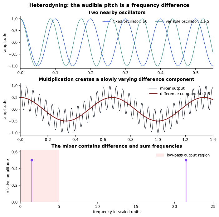
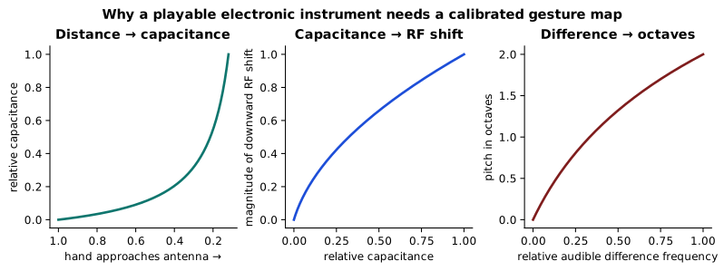
Source
ch02_heterodyne.py
assets/figures/src/ch02_heterodyne.pyPython
#!/usr/bin/env python3
"""Generate Chapter 2 heterodyne/control figures and gesture-listening audio."""

from __future__ import annotations

import wave
from pathlib import Path

import matplotlib
matplotlib.use("Agg")
import matplotlib.pyplot as plt
import numpy as np

ROOT = Path(__file__).resolve().parents[3]
SVG = ROOT / "assets/figures/svg"
AUDIO = ROOT / "assets/audio/ch02"
SVG.mkdir(parents=True, exist_ok=True)
AUDIO.mkdir(parents=True, exist_ok=True)

plt.rcParams.update(
    {
        "font.family": "DejaVu Sans",
        "font.size": 9,
        "axes.spines.top": False,
        "axes.spines.right": False,
        "axes.titleweight": "bold",
        "svg.fonttype": "none",
    }
)
RED = "#7F1D1D"
TEAL = "#0F766E"
BLUE = "#1D4ED8"
PURPLE = "#7C3AED"


def normalize_rms(signal: np.ndarray, target: float = 0.17) -> np.ndarray:
    signal = signal - np.mean(signal)
    rms = np.sqrt(np.mean(signal**2))
    return signal * (target / rms) if rms else signal


def fade(signal: np.ndarray, sample_rate: int, seconds: float = 0.03) -> np.ndarray:
    frames = min(int(sample_rate * seconds), len(signal) // 2)
    ramp = np.linspace(0.0, 1.0, frames)
    signal = signal.copy()
    signal[:frames] *= ramp
    signal[-frames:] *= ramp[::-1]
    return signal


def write_wav(path: Path, signal: np.ndarray, sample_rate: int = 48_000) -> None:
    signal = np.clip(signal, -0.98, 0.98)
    pcm = np.round(signal * 32767).astype("<i2")
    with wave.open(str(path), "wb") as output:
        output.setnchannels(1)
        output.setsampwidth(2)
        output.setframerate(sample_rate)
        output.writeframes(pcm.tobytes())


# Figure 1: scaled heterodyne example. Frequencies are deliberately low enough to see.
t = np.linspace(0.0, 1.4, 6000, endpoint=False)
f_fixed = 10.0
f_variable = 11.5
fixed = np.cos(2 * np.pi * f_fixed * t)
variable = np.cos(2 * np.pi * f_variable * t)
mixed = fixed * variable
low_component = 0.5 * np.cos(2 * np.pi * (f_variable - f_fixed) * t)
high_component = 0.5 * np.cos(2 * np.pi * (f_variable + f_fixed) * t)

fig, axes = plt.subplots(3, 1, figsize=(7.2, 7.1), constrained_layout=True)
axes[0].plot(t, fixed, color=BLUE, linewidth=0.9, label="fixed oscillator: 10")
axes[0].plot(t, variable, color=TEAL, linewidth=0.9, alpha=0.85, label="variable oscillator: 11.5")
axes[0].set_xlim(0, 0.55)
axes[0].set_ylabel("amplitude")
axes[0].set_title("Two nearby oscillators")
axes[0].legend(loc="upper right", frameon=False, ncol=2)

axes[1].plot(t, mixed, color="#111827", linewidth=0.75, label="mixer output")
axes[1].plot(t, low_component, color=RED, linewidth=1.8, label="difference component: 1.5")
axes[1].set_xlim(0, 1.4)
axes[1].set_ylabel("amplitude")
axes[1].set_title("Multiplication creates a slowly varying difference component")
axes[1].legend(loc="upper right", frameon=False)

markerline, stemlines, baseline = axes[2].stem(
    [f_variable - f_fixed, f_variable + f_fixed], [0.5, 0.5], basefmt=" "
)
plt.setp(markerline, color=PURPLE, markersize=5)
plt.setp(stemlines, color=PURPLE, linewidth=1.5)
axes[2].axvspan(0, 5, color="#FEE2E2", alpha=0.8, label="low-pass output region")
axes[2].set_xlim(0, 25)
axes[2].set_ylim(0, 0.62)
axes[2].set_xlabel("frequency in scaled units")
axes[2].set_ylabel("relative amplitude")
axes[2].set_title("The mixer contains difference and sum frequencies")
axes[2].legend(loc="upper right", frameon=False)
fig.suptitle("Heterodyning: the audible pitch is a frequency difference", fontsize=12, fontweight="bold")
fig.savefig(SVG / "ch02-heterodyne-principle.svg", bbox_inches="tight")
plt.close(fig)

# Figure 2: idealized control chain. The capacitance curve is a teaching analogy, not a theremin calibration.
distance = np.linspace(0.12, 1.0, 500)
capacitance = 1.0 / distance
capacitance = (capacitance - capacitance.min()) / (capacitance.max() - capacitance.min())
downward_shift_magnitude = np.sqrt(capacitance + 0.03)
downward_shift_magnitude = (
    (downward_shift_magnitude - downward_shift_magnitude.min())
    / (downward_shift_magnitude.max() - downward_shift_magnitude.min())
)
pitch_octaves = np.log2(1.0 + 3.0 * downward_shift_magnitude)

fig, axes = plt.subplots(1, 3, figsize=(8.2, 3.0), constrained_layout=True)
axes[0].plot(distance, capacitance, color=TEAL, linewidth=2)
axes[0].invert_xaxis()
axes[0].set(xlabel="hand approaches antenna →", ylabel="relative capacitance", title="Distance → capacitance")
axes[1].plot(capacitance, downward_shift_magnitude, color=BLUE, linewidth=2)
axes[1].set(
    xlabel="relative capacitance",
    ylabel="magnitude of downward RF shift",
    title="Capacitance → RF shift",
)
axes[2].plot(downward_shift_magnitude, pitch_octaves, color=RED, linewidth=2)
axes[2].set(
    xlabel="relative audible difference frequency",
    ylabel="pitch in octaves",
    title="Difference → octaves",
)
fig.suptitle("Why a playable electronic instrument needs a calibrated gesture map", fontsize=11, fontweight="bold")
fig.savefig(SVG / "ch02-gesture-to-pitch.svg", bbox_inches="tight")
plt.close(fig)

# Listening file: steady tone, portamento, vibrato, and independent volume articulation.
sample_rate = 48_000
silence = np.zeros(int(sample_rate * 0.4))
segments = []

def expressive_tone(frequency: np.ndarray, amplitude: np.ndarray) -> np.ndarray:
    phase = 2 * np.pi * np.cumsum(frequency) / sample_rate
    tone = np.sin(phase) + 0.22 * np.sin(2 * phase) + 0.08 * np.sin(3 * phase)
    return normalize_rms(tone * amplitude)

# Steady reference.
duration = 2.0
time = np.arange(int(sample_rate * duration)) / sample_rate
segments += [fade(expressive_tone(np.full_like(time, 330.0), np.ones_like(time)), sample_rate), silence]

# Continuous glissando: interpolation in log-frequency gives equal octave motion.
duration = 3.0
time = np.arange(int(sample_rate * duration)) / sample_rate
frequency = 220.0 * np.power(660.0 / 220.0, time / duration)
segments += [fade(expressive_tone(frequency, np.ones_like(time)), sample_rate), silence]

# Vibrato, ±25 cents around A4.
duration = 3.0
time = np.arange(int(sample_rate * duration)) / sample_rate
cents = 25.0 * np.sin(2 * np.pi * 5.5 * time)
frequency = 440.0 * np.power(2.0, cents / 1200.0)
segments += [fade(expressive_tone(frequency, np.ones_like(time)), sample_rate), silence]

# Independent amplitude articulation while pitch stays steady.
duration = 3.0
time = np.arange(int(sample_rate * duration)) / sample_rate
amplitude = np.clip(0.5 + 0.48 * np.sin(2 * np.pi * 1.2 * time - np.pi / 2), 0.02, 1.0)
segments += [fade(expressive_tone(np.full_like(time, 392.0), amplitude), sample_rate)]

write_wav(AUDIO / "ch02-continuous-control-studies.wav", np.concatenate(segments), sample_rate)
print("Generated Chapter 2 figures and audio.")
SOURCE AND OUTPUT
Equation figures
One deterministic Python program renders the exact plots paired with the numbered formulas. Equation 2.2 is rendered by the heterodyne program above.
Output
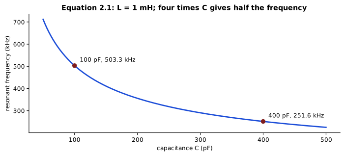
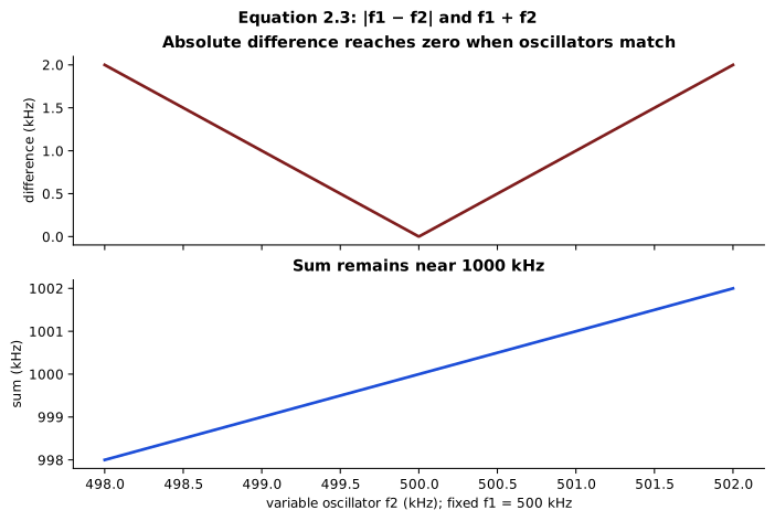
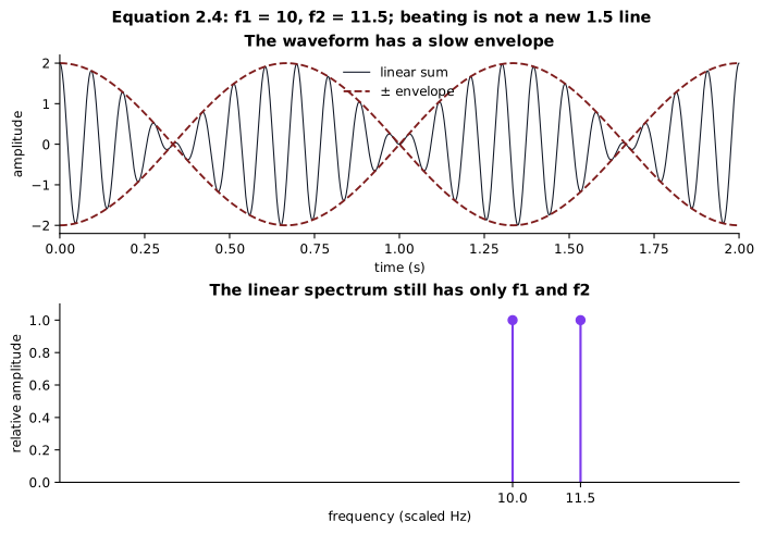
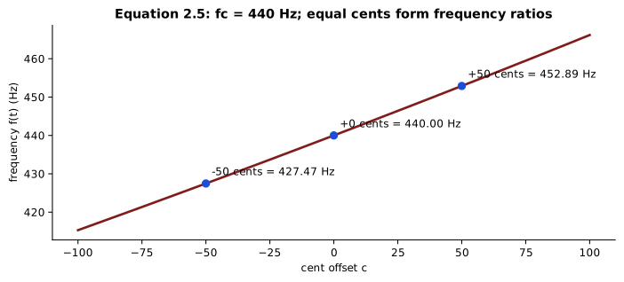
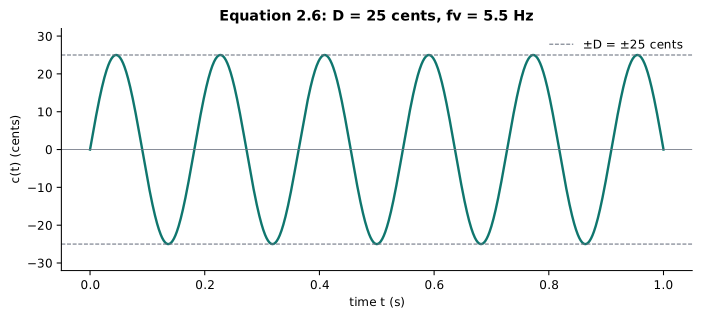
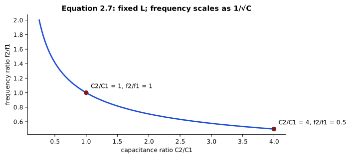
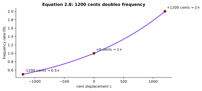
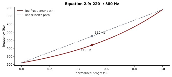
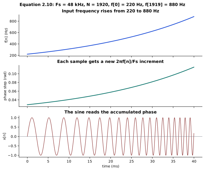
Source
formula_visuals_ch02.py
assets/figures/src/formula_visuals_ch02.pyPython
#!/usr/bin/env python3
"""Generate deterministic visuals for the numbered formulas in Chapter 2."""

from __future__ import annotations

from pathlib import Path

import matplotlib

matplotlib.use("Agg")
import matplotlib.pyplot as plt
import numpy as np

ROOT = Path(__file__).resolve().parents[3]
SVG = ROOT / "assets/figures/svg"
SVG.mkdir(parents=True, exist_ok=True)

RED = "#7F1D1D"
TEAL = "#0F766E"
BLUE = "#1D4ED8"
PURPLE = "#7C3AED"
GOLD = "#B45309"
GRAY = "#6B7280"
BLACK = "#111827"

plt.rcParams.update(
    {
        "font.family": "DejaVu Sans",
        "font.size": 9,
        "axes.spines.top": False,
        "axes.spines.right": False,
        "axes.titleweight": "bold",
        "svg.fonttype": "none",
    }
)


def save(fig: plt.Figure, filename: str) -> None:
    fig.savefig(SVG / filename, bbox_inches="tight")
    plt.close(fig)


def zero_line(axis: plt.Axes) -> None:
    axis.axhline(0.0, color=GRAY, linewidth=0.6)


# Equation 2.1: LC resonance falls as capacitance rises.
inductance = 1e-3
capacitance_pf = np.linspace(50.0, 500.0, 900)
capacitance_f = capacitance_pf * 1e-12
lc_frequency_khz = 1.0 / (2 * np.pi * np.sqrt(inductance * capacitance_f)) / 1000
fig, axis = plt.subplots(figsize=(7.2, 3.2), constrained_layout=True)
axis.plot(capacitance_pf, lc_frequency_khz, color=BLUE, linewidth=2)
for c_pf in [100.0, 400.0]:
    f_khz = 1.0 / (2 * np.pi * np.sqrt(inductance * c_pf * 1e-12)) / 1000
    axis.scatter([c_pf], [f_khz], color=RED, zorder=3)
    axis.annotate(f"{c_pf:.0f} pF, {f_khz:.1f} kHz", (c_pf, f_khz), xytext=(8, 6), textcoords="offset points")
axis.set(xlabel="capacitance C (pF)", ylabel="resonant frequency (kHz)", title="Equation 2.1: L = 1 mH; four times C gives half the frequency")
save(fig, "eq-2-1-lc-frequency.svg")

# Equation 2.3: difference and sum move differently as one oscillator moves.
fixed_khz = 500.0
variable_khz = np.linspace(498.0, 502.0, 900)
difference_khz = np.abs(fixed_khz - variable_khz)
sum_khz = fixed_khz + variable_khz
fig, axes = plt.subplots(2, 1, figsize=(7.2, 4.8), sharex=True, constrained_layout=True)
axes[0].plot(variable_khz, difference_khz, color=RED, linewidth=2)
axes[0].set(ylabel="difference (kHz)", title="Absolute difference reaches zero when oscillators match")
axes[1].plot(variable_khz, sum_khz, color=BLUE, linewidth=2)
axes[1].set(xlabel="variable oscillator f2 (kHz); fixed f1 = 500 kHz", ylabel="sum (kHz)", title="Sum remains near 1000 kHz")
fig.suptitle("Equation 2.3: |f1 − f2| and f1 + f2", fontweight="bold")
save(fig, "eq-2-3-sum-difference.svg")

# Equation 2.4: linear addition beats but keeps only the input spectrum lines.
f1 = 10.0
f2 = 11.5
t_beats = np.linspace(0.0, 2.0, 5000, endpoint=False)
linear_sum = np.cos(2 * np.pi * f1 * t_beats) + np.cos(2 * np.pi * f2 * t_beats)
envelope = 2 * np.cos(np.pi * (f2 - f1) * t_beats)
fig, axes = plt.subplots(2, 1, figsize=(7.2, 5.0), constrained_layout=True)
axes[0].plot(t_beats, linear_sum, color=BLACK, linewidth=0.8, label="linear sum")
axes[0].plot(t_beats, envelope, color=RED, linewidth=1.4, linestyle="--", label="± envelope")
axes[0].plot(t_beats, -envelope, color=RED, linewidth=1.4, linestyle="--")
axes[0].set(xlabel="time (s)", ylabel="amplitude", xlim=(0, 2), title="The waveform has a slow envelope")
axes[0].legend(frameon=False)
markerline, stemlines, _ = axes[1].stem([f1, f2], [1.0, 1.0], basefmt=" ")
plt.setp(markerline, color=PURPLE, markersize=6)
plt.setp(stemlines, color=PURPLE, linewidth=1.6)
axes[1].set(xlabel="frequency (scaled Hz)", ylabel="relative amplitude", xticks=[f1, f2], xlim=(0, 15), ylim=(0, 1.1), title="The linear spectrum still has only f1 and f2")
fig.suptitle("Equation 2.4: f1 = 10, f2 = 11.5; beating is not a new 1.5 line", fontweight="bold")
save(fig, "eq-2-4-linear-beating.svg")

# Equation 2.5: map cent offset to frequency around A4.
cents = np.linspace(-100.0, 100.0, 800)
center_hz = 440.0
mapped_hz = center_hz * np.power(2.0, cents / 1200.0)
fig, axis = plt.subplots(figsize=(7.2, 3.2), constrained_layout=True)
axis.plot(cents, mapped_hz, color=RED, linewidth=2)
for c in [-50.0, 0.0, 50.0]:
    f = center_hz * 2 ** (c / 1200)
    axis.scatter([c], [f], color=BLUE, zorder=3)
    axis.annotate(f"{c:+.0f} cents = {f:.2f} Hz", (c, f), xytext=(5, 7), textcoords="offset points")
axis.set(xlabel="cent offset c", ylabel="frequency f(t) (Hz)", title="Equation 2.5: fc = 440 Hz; equal cents form frequency ratios")
save(fig, "eq-2-5-cents-frequency.svg")

# Equation 2.6: sinusoidal vibrato in cent space.
t_vibrato = np.linspace(0.0, 1.0, 1600)
depth_cents = 25.0
vibrato_rate = 5.5
cent_trajectory = depth_cents * np.sin(2 * np.pi * vibrato_rate * t_vibrato)
fig, axis = plt.subplots(figsize=(7.2, 3.2), constrained_layout=True)
axis.plot(t_vibrato, cent_trajectory, color=TEAL, linewidth=1.8)
axis.axhline(depth_cents, color=GRAY, linestyle="--", linewidth=0.8, label="±D = ±25 cents")
axis.axhline(-depth_cents, color=GRAY, linestyle="--", linewidth=0.8)
zero_line(axis)
axis.set(xlabel="time t (s)", ylabel="c(t) (cents)", ylim=(-32, 32), title="Equation 2.6: D = 25 cents, fv = 5.5 Hz")
axis.legend(frameon=False)
save(fig, "eq-2-6-vibrato-cents.svg")

# Equation 2.7: LC frequency ratio as capacitance ratio changes.
capacitance_ratio = np.linspace(0.25, 4.0, 900)
frequency_ratio = np.sqrt(1.0 / capacitance_ratio)
fig, axis = plt.subplots(figsize=(7.2, 3.2), constrained_layout=True)
axis.plot(capacitance_ratio, frequency_ratio, color=BLUE, linewidth=2)
for ratio in [1.0, 4.0]:
    value = np.sqrt(1 / ratio)
    axis.scatter([ratio], [value], color=RED, zorder=3)
    axis.annotate(f"C2/C1 = {ratio:g}, f2/f1 = {value:g}", (ratio, value), xytext=(7, 7), textcoords="offset points")
axis.set(xlabel="capacitance ratio C2/C1", ylabel="frequency ratio f2/f1", title="Equation 2.7: fixed L; frequency scales as 1/√C")
save(fig, "eq-2-7-lc-ratio.svg")

# Equation 2.8: cents expressed directly as a frequency ratio.
cents_wide = np.linspace(-1200.0, 1200.0, 1200)
ratio = np.power(2.0, cents_wide / 1200.0)
fig, axis = plt.subplots(figsize=(7.2, 3.2), constrained_layout=True)
axis.plot(cents_wide, ratio, color=PURPLE, linewidth=2)
for c, r in [(-1200, 0.5), (0, 1.0), (1200, 2.0)]:
    axis.scatter([c], [r], color=RED, zorder=3)
    axis.annotate(f"{c:+d} cents → {r:g}×", (c, r), xytext=(5, 7), textcoords="offset points")
axis.set(xlabel="cent displacement c", ylabel="frequency ratio f/fc", title="Equation 2.8: 1200 cents doubles frequency")
save(fig, "eq-2-8-cents-ratio.svg")

# Equation 2.9: logarithmic and linear interpolation do not share a midpoint.
u = np.linspace(0.0, 1.0, 800)
start_hz = 220.0
end_hz = 880.0
log_path = start_hz * np.power(end_hz / start_hz, u)
linear_path = start_hz + (end_hz - start_hz) * u
fig, axis = plt.subplots(figsize=(7.2, 3.2), constrained_layout=True)
axis.plot(u, log_path, color=RED, linewidth=2, label="log-frequency path")
axis.plot(u, linear_path, color=GRAY, linewidth=1.4, linestyle="--", label="linear-hertz path")
axis.scatter([0.5, 0.5], [440, 550], color=[RED, GRAY], zorder=3)
axis.annotate("440 Hz", (0.5, 440), xytext=(-35, -18), textcoords="offset points")
axis.annotate("550 Hz", (0.5, 550), xytext=(8, 8), textcoords="offset points")
axis.set(xlabel="normalized progress u", ylabel="frequency (Hz)", title="Equation 2.9: 220 → 880 Hz")
axis.legend(frameon=False)
save(fig, "eq-2-9-log-interpolation.svg")

# Equation 2.10: frequency controls phase increment; accumulated phase controls the waveform.
sample_rate = 48_000
samples = 1_920
time = np.arange(samples) / sample_rate
progress = np.linspace(0.0, 1.0, samples)
frequency_path = 220.0 * np.power(880.0 / 220.0, progress)
increment = 2 * np.pi * frequency_path / sample_rate
phase_path = np.zeros(samples)
phase_path[1:] = np.cumsum(increment[:-1])
waveform = np.sin(phase_path)
assert frequency_path[0] == 220.0 and frequency_path[-1] == 880.0
assert phase_path[0] == 0.0
fig, axes = plt.subplots(3, 1, figsize=(7.2, 6.0), sharex=True, constrained_layout=True)
axes[0].plot(time * 1000, frequency_path, color=BLUE, linewidth=1.8)
axes[0].set(ylabel="f[n] (Hz)", title="Input frequency rises from 220 to 880 Hz")
axes[1].plot(time * 1000, increment, color=TEAL, linewidth=1.8)
axes[1].set(ylabel="phase step (rad)", title="Each sample gets a new 2πf[n]/Fs increment")
axes[2].plot(time * 1000, waveform, color=RED, linewidth=0.9)
zero_line(axes[2])
axes[2].set(xlabel="time (ms)", ylabel="x[n]", title="The sine reads the accumulated phase")
fig.suptitle("Equation 2.10: Fs = 48 kHz, N = 1920, f[0] = 220 Hz, f[1919] = 880 Hz", fontweight="bold")
save(fig, "eq-2-10-phase-accumulation.svg")

print("Generated Chapter 2 formula visuals.")
SOURCE AND OUTPUT
Theremin signal diagram
The Mermaid source produces the full control and heterodyne signal path.
Output
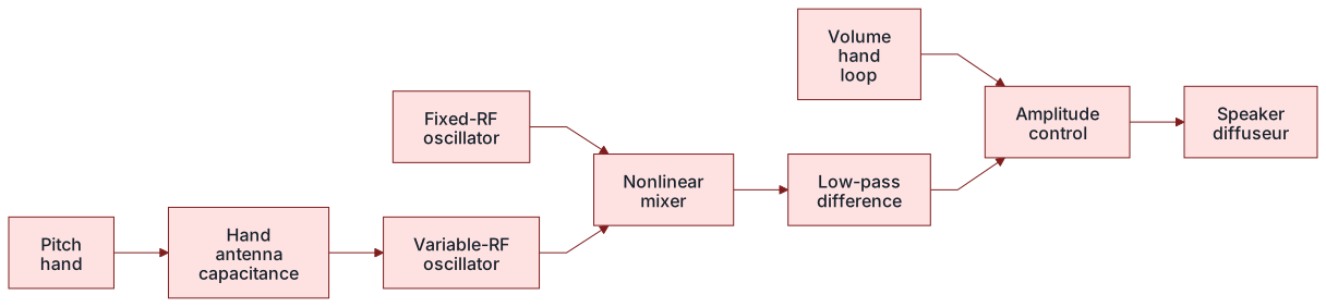
Source
ch02-heterodyne-instrument.mmd
assets/diagrams/src/ch02-heterodyne-instrument.mmdMermaid
flowchart LR
    HP[Pitch<br/>hand] --> CAP[Hand<br/>antenna<br/>capacitance]
    CAP --> VAR[Variable-RF<br/>oscillator]
    FIX[Fixed-RF<br/>oscillator] --> MIX[Nonlinear<br/>mixer]
    VAR --> MIX
    MIX --> LP[Low-pass<br/>difference]
    HV[Volume<br/>hand<br/>loop] --> AMP[Amplitude<br/>control]
    LP --> AMP
    AMP --> OUT[Speaker<br/>diffuseur]
Chapter 2 Answers and Fault Invariants
Chapter 2 mathematical-practice answers
- .
- Difference: 440 Hz. Sum: 519,560 Hz.
- Linear superposition retains spectral components at the two inputs. The 440 Hz envelope rate is not a new 440 Hz spectrum line; multiplication or another nonlinearity is required.
- Hz and Hz.
- Logarithmic midpoint: Hz. Linear midpoint: Hz.
- radians per sample. For a glide, recompute the increment from each and add it to the previous phase.
- Hz = 299.41267 kHz.
- A valid response identifies every axis or panel, copies the stated parameters, and links one visual feature to the formula. Examples include LC frequency falling with capacitance, multiplication creating two new lines, log interpolation reaching 440 Hz halfway, and phase steps increasing during the glide.
Chapter 2 readiness answers
- The variable LC oscillator falls because . Its distance from the fixed oscillator can increase, so the audible difference frequency rises.
- The nonlinear mixer produces 1 kHz and 1001 kHz. An audio low-pass filter retains 1 kHz.
- The trigonometric envelope of a linear sum varies, but its Fourier components remain at the original two frequencies. A nonlinear product generates cross-components at the sum and difference.
- At 0°, equal 220 Hz waves align and produce the same pitch at twice the peak amplitude, about 6.02 dB above one wave. At 180°, every value has an equal opposite and the ideal sum is silence.
- A passive real tank loses energy to resistance, dielectric loss, and radiation, so its amplitude trajectory decays. Correctly phased active feedback can replace approximately that loss each cycle and sustain a steady trajectory.
- The pitch hand controls capacitance near the vertical rod; the volume hand shapes amplitude near the loop. Amplitude control creates attack, release, separation, accent, and rest instead of exposing every pitch movement continuously.
- Vibrato is periodic pitch motion around a target; portamento is continuous travel between targets; articulation shapes onset, connection, emphasis, and release, commonly through amplitude.
- Mobile keyboard and ring/wire. The intensity key provides pressure-shaped amplitude and articulation. A resonant diffuser changes spectral colour and decay rather than only increasing level.
Chapter 2 faded and musical-station invariants
- Variable frequencies below 300.000 kHz are 299.56000 kHz for A4, 299.47675 kHz for C5, and 299.34075 kHz for E5.
- As the target audio frequency rises, the below-fixed variable oscillator moves farther downward.
- The low-pass stage must reject the RF sum and other high-frequency mixer products.
- Acceptable musical proof contains separate pitch and amplitude trajectories, two contrasting articulations of the same pitch centers, and a listener observation about event clarity versus continuity.
Chapter 2 fault invariant
- The antenna is primarily a capacitive proximity electrode, not a blocked beam.
- Increased capacitance lowers LC frequency directly.
- Linear addition is not nonlinear heterodyne mixing.
- The Ondes adds distinct pitch interfaces, haptic amplitude control, timbre selection, and specialized outputs; it is not merely a keyed theremin.